Create occurrence cubes for virtual species

Apart from simulating occurrence cubes from scratch, gcube can also be used to create cubes for virtual species generated using bioclimatic variables. This tutorial demonstrates how to generate a virtual species, apply a geographical limit, sample occurrences, and convert them into an occurrence cube.

Create virtual species

Virtual species can be created using the virtualspecies R package (Leroy et al., 2015). Below is a basic example of how to create a virtual species. For additional options and a more comprehensive guide, refer to the package documentation and the tutorial available here.

# Load packages
library(gcube)

library(geodata)        # get bioclimatic data
library(virtualspecies) # generate virtual species

library(sf)             # work with spatial objects
library(terra)          # work with raster data
library(ggplot2)        # data visualisation

Step 1: Download WorldClim Data

We first obtain WorldClim bioclimatic data at a 10-minute resolution.

# Download bioclimatic data
worldclim <- worldclim_global(var = "bio", res = 10, path = tempdir())

Step 2: Define the region of interest

We define the extent for the Western Palearctic and crop the climate data.

# Western Palearctic
wp <- terra::ext(-15, 65, 30, 75)

# Crop climate data
worldclim <- terra::crop(worldclim, wp)

Step 3: Select relevant bioclimatic variables

We select a subset of bioclimatic variables: bio2, bio5, bio6, bio13, bio14, and bio15.

# Specify variables
bio_vars <- c("bio2", "bio5", "bio6", "bio13", "bio14", "bio15")

# Select variables
bio_string <- paste0("bio_", sub("bio", "", bio_vars), collapse = "|")
bio_vars_selected <- names(worldclim)[grepl(bio_string, names(worldclim))]

# Subset climate data
worldclim_vars <- worldclim[[bio_vars_selected]]

Step 4: Generate a virtual species

We create a random virtual species based on the selected bioclimatic variables.

set.seed(123)

# Generate random virtual species
virtual_species <- generateRandomSp(worldclim_vars)
#> Reading raster values. If it fails for very large rasters, use arguments 'sample.points = TRUE' and define a number of points to sample with 'nb.point'.
#>  - Perfoming the pca
#>  - Defining the response of the species along PCA axes
#>  - Calculating suitability values
#>    The final environmental suitability was rescaled between 0 and 1.
#>                   To disable, set argument rescale = FALSE
#>  - Converting into Presence - Absence
#>    --- Generating a random value of beta for the logistic conversion
#>    --- Determing species.prevalence automatically according to alpha and beta
#>    Logistic conversion finished:
#>               
#> - beta = 0.194194194194194
#> - alpha = -0.1
#> - species prevalence =0.770632849948426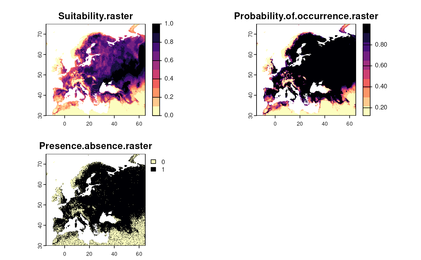

Step 5: Apply a geographical limit

We limit the species distribution to the United Kingdom and Ireland.

# Limit distribution
virtual_distribution <- limitDistribution(
  x = virtual_species,
  geographical.limit = "country",
  area = c("United Kingdom", "Ireland")
)
#> Warning: [rasterize] unexpected additional argument(s): silent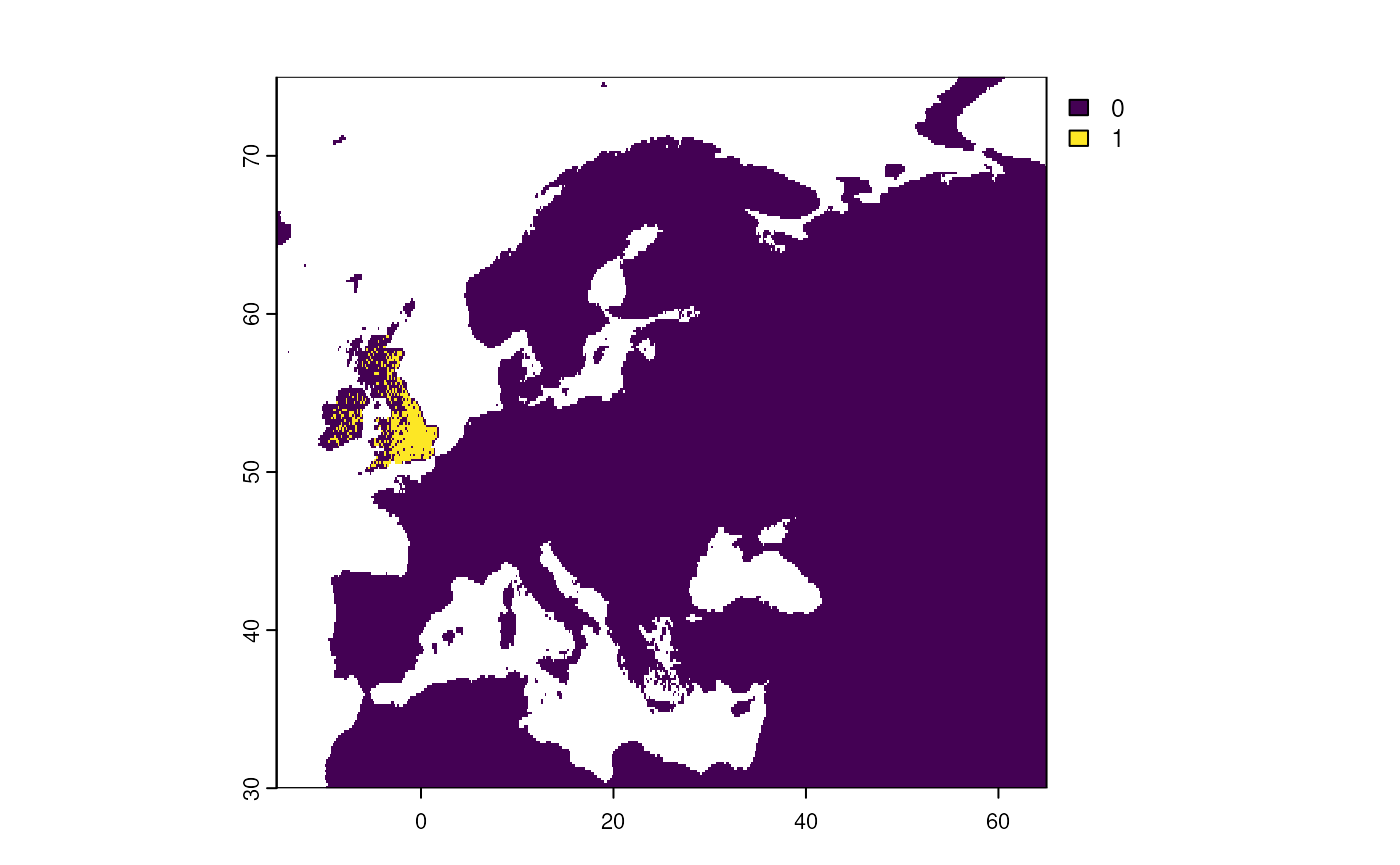

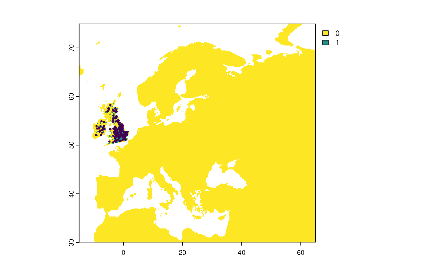
Step 6: Sample occurrences

We sample 150 occurrences from the restricted distribution with a detection probability of 0.8 using the virtualspecies::sampleOccurrences() function. Detection probability and sampling bias can be introduced similar to sample_observations().

?virtualspecies::sampleOccurrences

# Sample from virtual species distribution
virtual_sample <- sampleOccurrences(
  virtual_distribution,
  n = 150,
  detection.probability = 0.8
)

Grid designation with gcube

Now we can create an occurrence cube for this virtual species The most important step, is to make the virtualspecies output compatible with gcube input. This is done using the virtualsample_to_sf() function.

For grid designation, see also the tutorial 3. Specifying the grid designation process.

Step 1: Convert sampled points to sf format

We transform the sampled points from a virtualspecies object so that it can be used by gcube with the virtualsample_to_sf() function.

?virtualsample_to_sf

# Transform virtual samples to sf object
detections_df_raw <- virtualsample_to_sf(virtual_sample)
detections_df_raw
#> Simple feature collection with 150 features and 2 fields
#> Geometry type: POINT
#> Dimension:     XY
#> Bounding box:  xmin: -9.25 ymin: 50.58333 xmax: 1.416667 ymax: 58.25
#> Geodetic CRS:  WGS 84
#> First 10 features:
#>       id observed                    geometry
#> 1  62966     TRUE      POINT (-0.75 53.08333)
#> 2  60516     TRUE  POINT (-9.083333 53.91667)
#> 3  63937     TRUE      POINT (1.083333 52.75)
#> 4  59607     TRUE    POINT (-0.5833333 54.25)
#> 5  66802     TRUE     POINT (-1.416667 51.75)
#> 6  65795     TRUE      POINT (-9.25 52.08333)
#> 7  60087     TRUE POINT (-0.5833333 54.08333)
#> 8  55755     TRUE  POINT (-2.583333 55.58333)
#> 9  54310     TRUE  POINT (-3.416667 56.08333)
#> 10 56230     TRUE  POINT (-3.416667 55.41667)

---

Optional: Extract values from a raster

You can also extract raster values when transforming the sample data. For instance, extracting suitability or occurrence probability can be helpful for downstream analysis.

# Rename raster layers for clear output
names(virtual_species$suitab.raster) <- "suitability"
names(virtual_species$probability.of.occurrence) <- "occ_prob"

# Transform virtual samples and extract values
virtualsample_to_sf(
  virtual_sample,
  raster_lyr = c(virtual_species$suitab.raster,
                 virtual_species$probability.of.occurrence)
)
#> Simple feature collection with 150 features and 4 fields
#> Geometry type: POINT
#> Dimension:     XY
#> Bounding box:  xmin: -9.25 ymin: 50.58333 xmax: 1.416667 ymax: 58.25
#> Geodetic CRS:  WGS 84
#> First 10 features:
#>       id observed suitability  occ_prob                    geometry
#> 1  62966     TRUE 0.608657235 0.9843980      POINT (-0.75 53.08333)
#> 2  60516     TRUE 0.081922322 0.2455073  POINT (-9.083333 53.91667)
#> 3  63937     TRUE 0.481108846 0.9463000      POINT (1.083333 52.75)
#> 4  59607     TRUE 0.375077019 0.8592202    POINT (-0.5833333 54.25)
#> 5  66802     TRUE 0.516553006 0.9617124     POINT (-1.416667 51.75)
#> 6  65795     TRUE 0.019556962 0.1485053      POINT (-9.25 52.08333)
#> 7  60087     TRUE 0.354688757 0.8327085 POINT (-0.5833333 54.08333)
#> 8  55755     TRUE 0.294534380 0.7317269  POINT (-2.583333 55.58333)
#> 9  54310     TRUE 0.248244943 0.6319305  POINT (-3.416667 56.08333)
#> 10 56230     TRUE 0.004863729 0.1308681  POINT (-3.416667 55.41667)

---

We transform the detected points into an sf object to the LAEA Europe CRS (EPSG:3035).

# Transform CRS
detections_df_transformed <- st_transform(detections_df_raw, crs = 3035)

Step 2: Add coordinate uncertainty

See also the tutorial 2. Simulating the detection process.

We only keep the detected occurrences using the filter_observations() function.

detections_df <- filter_observations(detections_df_transformed)

Optionally, we can add coordinate uncertainty using the add_coordinate_uncertainty() function. We add 25 m uncertainty for each observation.

# Add coordinate uncertainty
observations_df <- add_coordinate_uncertainty(
  observations = detections_df,
  coords_uncertainty_meters = 25
)

Step 3: Specify reference grid

We also need a grid. Each observation will be designated to a grid cell. You can provide your own grid (e.g. EEA reference grid for Europe). For this example we create a simple grid around the sampled points.

# Create reference grid
buffered_observations <- st_buffer(observations_df, 25)
cube_grid <- st_make_grid(
  buffered_observations,
  n = c(20, 20),
  square = TRUE
) %>%
  st_sf()

The grid looks like this.

ggplot() +
  geom_sf(data = observations_df) +
  geom_sf(data = cube_grid, alpha = 0) +
  coord_sf(datum = 3035) +
  theme_minimal()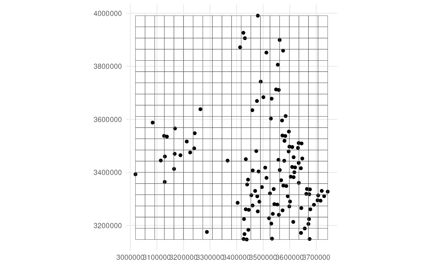

Step 4: Perform grid designation

We perform grid designation both in aggregated version and not for visualisation purposes.

# Perform grid designation
occurrence_cube_df <- grid_designation(
  observations_df,
  cube_grid,
  seed = 123
)
#> Warning in sample_from_uniform_circle(observations = observations, missing_uncertainty = missing_uncertainty, : No column `time_point` present!
#> Assuming only a single time point.

# Get sampled points from uncertainty circle
sampled_points <- grid_designation(
  observations_df,
  cube_grid,
  seed = 123,
  aggregate = FALSE
)
#> Warning in sample_from_uniform_circle(observations = observations, missing_uncertainty = missing_uncertainty, : No column `time_point` present!
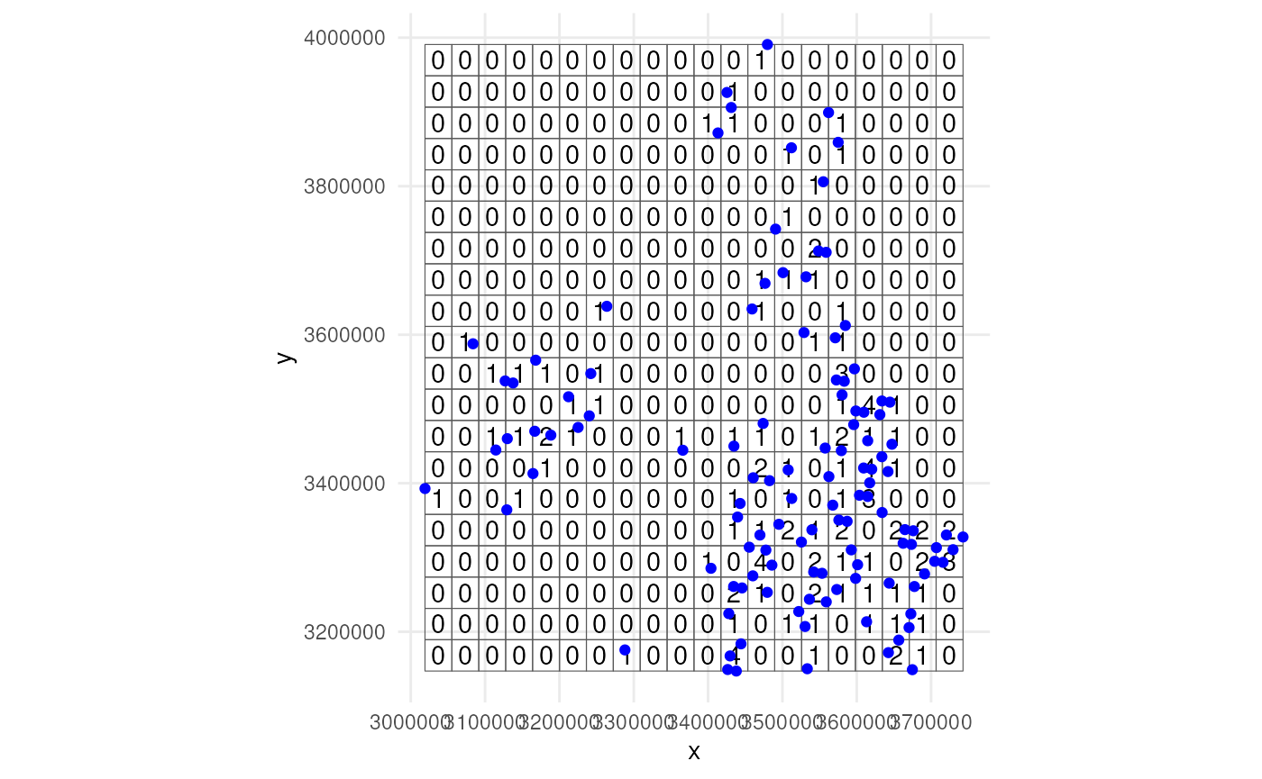
#> Assuming only a single time point.

Lets visualise were the samples were taken. Note that no distinction is made between zeroes and NA values. Every absence gets a zero value.

ggplot() +
  geom_sf(data = occurrence_cube_df,
          alpha = 0) +
  geom_sf_text(data = occurrence_cube_df,
               aes(label = n)) +
  geom_sf(data = sampled_points,
          colour = "blue") +
  coord_sf(datum = 3035) +
  theme_minimal()