2. Simulating the detection process

The workflow for simulating a biodiversity data cube used in gcube can be divided in three steps or processes:

1. Occurrence process
2. Detection process
3. Grid designation process

This tutorial documents the second part of the gcube simulation workflow, viz. the detection process.

# Load packages
library(gcube)

library(sf)        # work with spatial objects
library(dplyr)     # data wrangling
library(ggplot2)   # data visualisation

Input

The functions are set up such that a single polygon as input is enough to go through this workflow using default arguments. The user can change these arguments to allow for more flexibility.

As input, we create a polygon in which we simulate occurrences. It represents the spatial extend of the species.

polygon <- st_polygon(list(cbind(c(500, 1000, 1000, 600, 200, 100, 500),
                                 c(200, 100, 700, 1000, 900, 500, 200))))

The polygon looks like this.

ggplot() +
  geom_sf(data = polygon) +
  theme_minimal()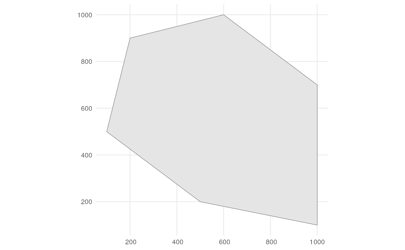

We can for example sample randomly within the polygon over 6 time points were we use a random walk over time with an initial average number of occurrences equal to 100 (see see tutorial 1 about simulating the occurrence process).

occurrences_df <- simulate_occurrences(
  species_range = polygon,
  initial_average_occurrences = 100,
  n_time_points = 6,
  temporal_function = simulate_random_walk,
  sd_step = 1,
  spatial_pattern = "random",
  seed = 123)
#> [using unconditional Gaussian simulation]

This is the spatial distribution of the occurrences for each time point

ggplot() +
  geom_sf(data = polygon) +
  geom_sf(data = occurrences_df) +
  facet_wrap(~time_point, nrow = 2) +
  ggtitle("Distribution of occurrences for each time point") +
  theme_minimal()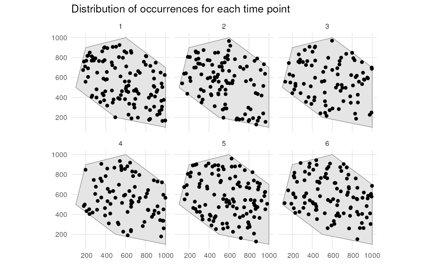

Detect occurrences

We have our occurrences, but not all occurrences are generally observed. The detection of occurrences depends on the detection probability of a species and the sampling bias (includes both sampling bias and effort). This process can be simulated using the sample_observations() function.

?sample_observations

Each observation will have a detection probability value (=the same for all observations) and a bias weight depending on its spatial distribution. The combination of detection probability and bias weight results in a sampling probability which is used to decide whether each occurrence is detected or not using (rbinom(1, 1, sampling_probability)).

For bias there are 3 options: "no_bias", "polygon" or "manual".

1. With "no_bias", only the detection probability value will decide whether an occurrence is observed or not.
2. With "polygon", bias weights depend on their location inside or outside a given polygon with a certain bias strength. We can visualise this using the supporting function apply_polygon_sampling_bias().

?apply_polygon_sampling_bias

Lets say we have a road across our polygon. Define the road width.

road_width <- 50

Create road points.

road_points <- rbind(c(100, 500), c(1000, 500))

Create road-like polygon within the given polygon.

road_polygon <- st_linestring(road_points) %>%
  st_buffer(road_width) %>%
  st_intersection(polygon) %>%
  st_polygon() %>%
  st_sfc() %>%
  st_as_sf() %>%
  rename(geometry = x)

Plot the result.

ggplot() +
  geom_sf(data = polygon, fill = "lightgreen") +
  geom_sf(data = road_polygon) +
  theme_minimal()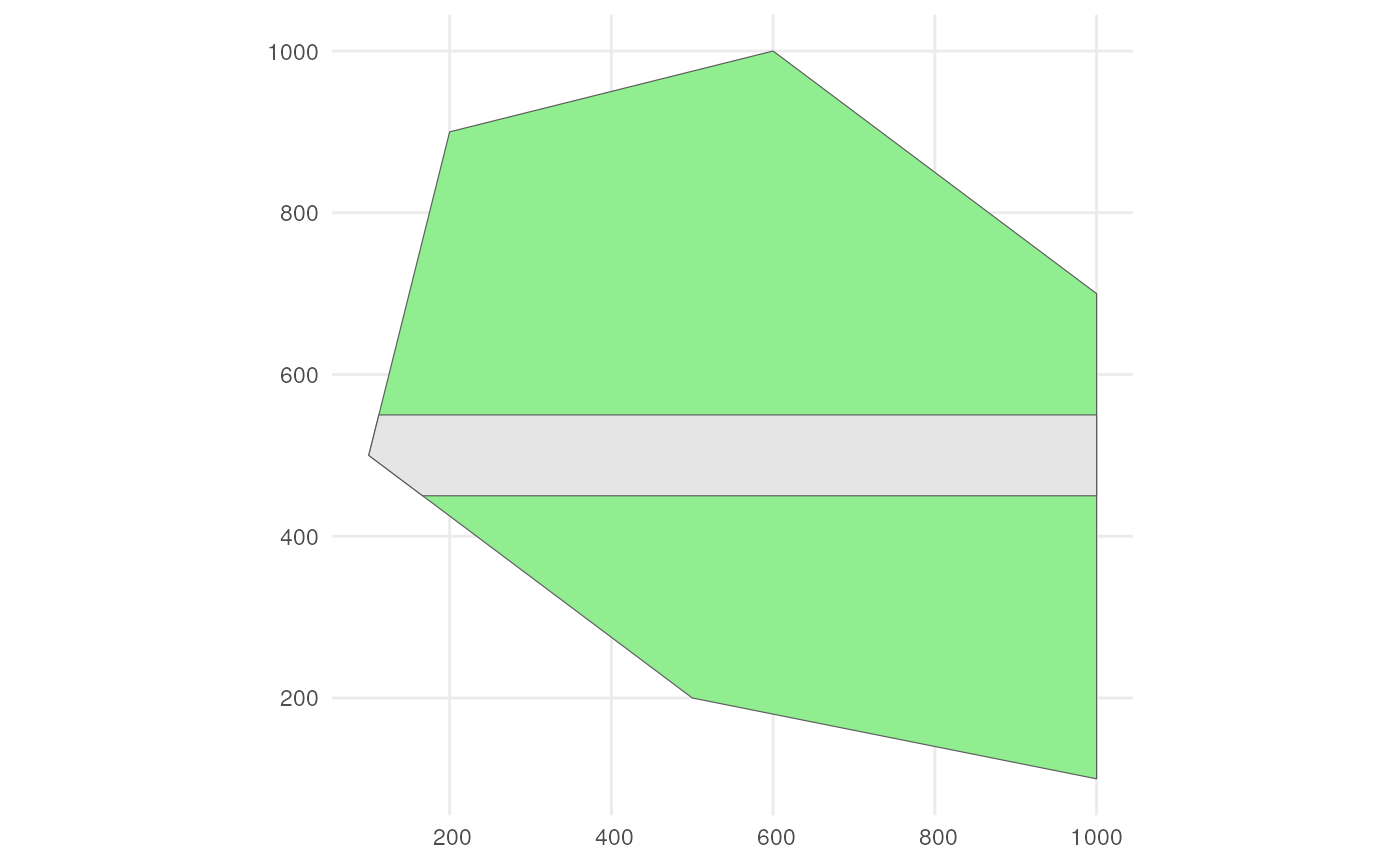

We can say that occurrences on the road have 2x larger probability to be detected.

occurrence_bias_df1 <- apply_polygon_sampling_bias(
  occurrences_df,
  bias_area = road_polygon,
  bias_strength = 2)

We see that occurrences on the road have twice the bias weights as the other occurrences.

ggplot() +
  geom_sf(data = polygon, fill = "lightgreen") +
  geom_sf(data = road_polygon) +
  geom_sf(data = occurrence_bias_df1,
          aes(colour = factor(round(bias_weight, 3)))) +
  facet_wrap(~time_point, nrow = 2) +
  labs(title = "Distribution of occurrences for each time point",
       colour = "bias_weight") +
  theme_minimal()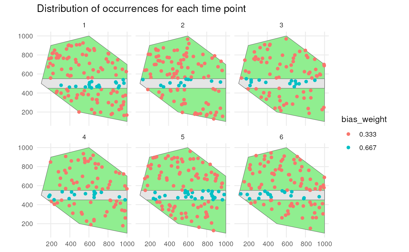

3. With "manual", bias weights depend on their location inside grid cells of a given grid where each cell has its own value. We can visualise this using the supporting function apply_manual_sampling_bias().

?apply_manual_sampling_bias

Lets create a grid and give random bias weights to each cell.

grid <- st_make_grid(
    polygon,
    n = c(10, 10),
    square = TRUE) %>%
  st_sf()
set.seed(123)
grid$bias_weight <- runif(nrow(grid), min = 0, max = 1)

Plot the grid.

ggplot() +
  geom_sf(data = polygon) +
  geom_sf(data = grid, alpha = 0) +
  geom_sf_text(data = grid, aes(label = round(bias_weight, 2))) +
  theme_minimal()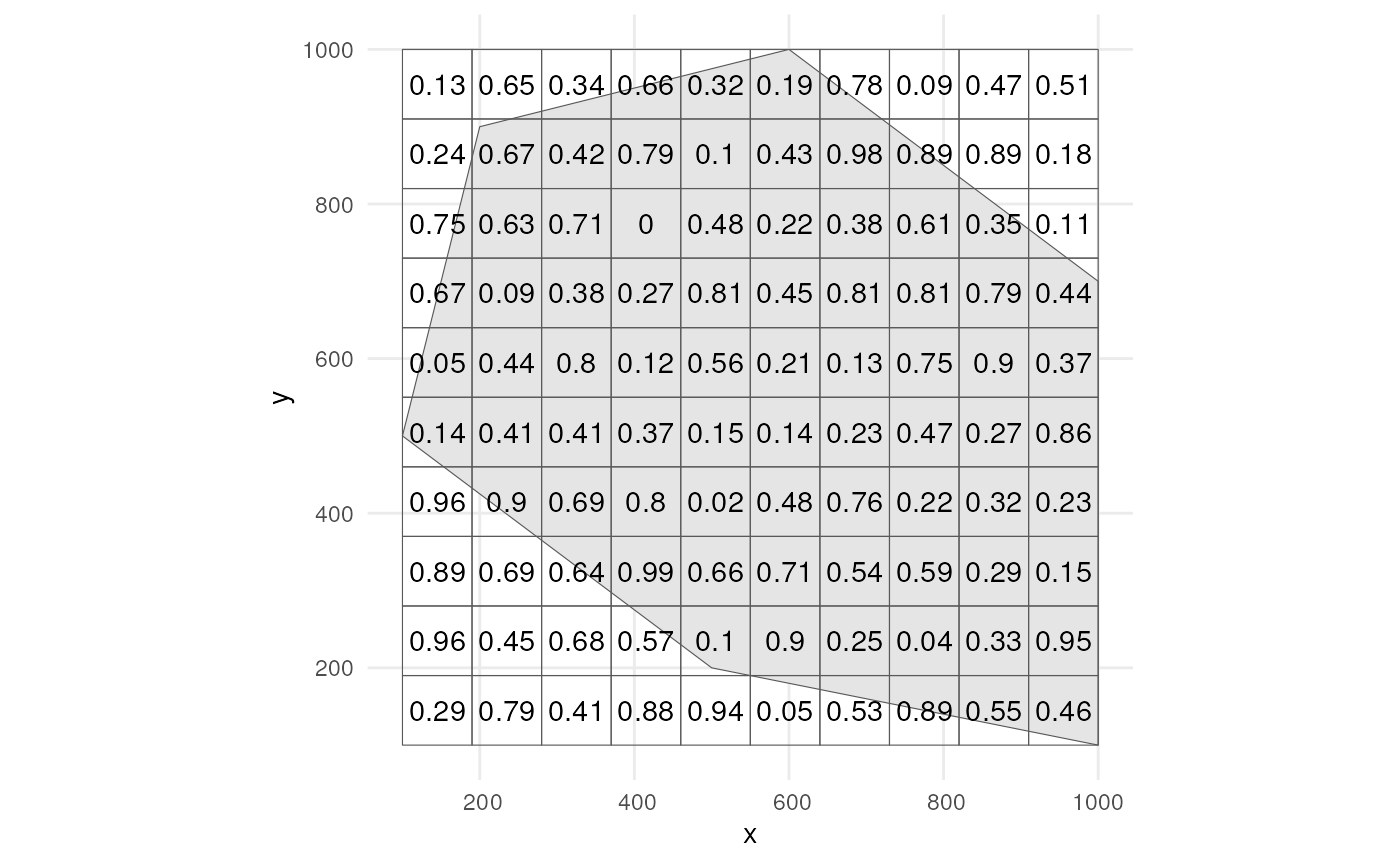

We use the supporting function. We only use time point 1.

occurrence_bias_df2 <- apply_manual_sampling_bias(
  occurrences_df %>% dplyr::filter(time_point == 1),
  bias_weights = grid)

We indeed see higher bias weights for occurrences where with higher values in the grid cells.

ggplot() +
  geom_sf(data = polygon) +
  geom_sf(data = grid, alpha = 0) +
  geom_sf(data = occurrence_bias_df2,
          aes(colour = bias_weight)) +
  geom_sf_text(data = grid, aes(label = round(bias_weight, 2))) +
  theme_minimal()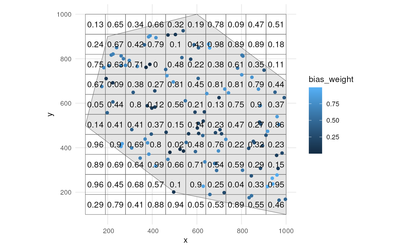

Example

Now that we know how the supporting functions work, we can simulate the detection process using the sample_observations() function. We can for example state that our species has a 0.9 detection probability and this time we say there is a very small chance to detect it on the road.

detections_df_raw <- sample_observations(
  occurrences_df,
  detection_probability = 0.9,
  sampling_bias = "polygon",
  bias_area = road_polygon,
  bias_strength = 0.1,
  seed = 123)

We see that a lot of occurrences are detected due to the high detection probability, but this is not the case on the road where few are detected.

ggplot() +
  geom_sf(data = polygon, fill = "lightgreen") +
  geom_sf(data = road_polygon) +
  geom_sf(data = detections_df_raw,
          aes(colour = sampling_status)) +
  scale_colour_manual(values = c("blue", "red")) +
  facet_wrap(~time_point, nrow = 2) +
  labs(title = "Distribution of occurrences for each time point") +
  theme_minimal()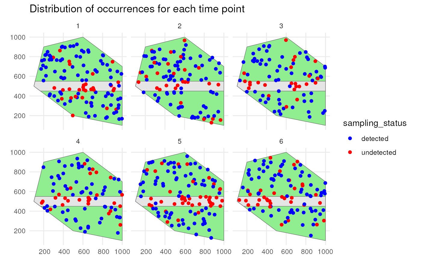

Adding coordinate uncertainty

To mimic real life data collection, we can finally add coordinate uncertainty to our observations. We only keep the detected occurrences of the previous example. We can filter with dplyr::filter().

detections_df1 <- detections_df_raw %>%
  dplyr::filter(sampling_status == "detected")

Or we can use the function filter_observations().

?filter_observations

detections_df2 <- filter_observations(
  observations_total = detections_df_raw)

# Do we get the same result?
identical(detections_df1, detections_df2)
#> [1] TRUE

We add coordinate uncertainty to the observations using the add_coordinate_uncertainty() function.

?add_coordinate_uncertainty

You can add a value for all observations or a vector with a single value for each observation. Lets add 25 meters of uncertainty to each observation.

observations_df <- add_coordinate_uncertainty(
  observations = detections_df2,
  coords_uncertainty_meters = 25)

Created and sf object with uncertainty circles to visualise this.

buffered_observations <- st_buffer(
  observations_df,
  observations_df$coordinateUncertaintyInMeters)

ggplot() +
  geom_sf(data = polygon, fill = "lightgreen") +
  geom_sf(data = road_polygon) +
  geom_sf(data = buffered_observations,
          fill = alpha("firebrick", 0.3)) +
  geom_sf(data = observations_df, colour = "firebrick", size = 0.8) +
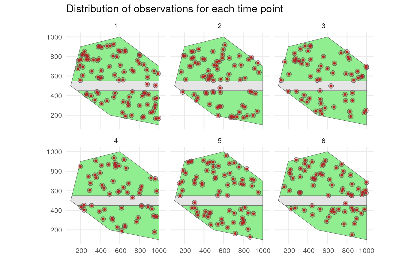
  facet_wrap(~time_point, nrow = 2) +
  labs(title = "Distribution of observations for each time point") +
  theme_minimal()