Invasion fitness synthesis

---

Install and load invasimapr and other core packages

Install from GitHub (recommended for development) or CRAN (if available) as before.

---

Synthesising invasion-fitness insights

This section condenses the high-dimensional output into system-level distributions, top/bottom ranks, trait correlates, and key-invader maps. The goal is a compact dashboard for reporting and decision-support.

:hourglass_flowing_sand: Step-by-step in this section:

1. Summarise the distribution of \(\lambda_{is}\),
2. Identify top/bottom invaders and sites by mean fitness,
3. Link invader traits to fitness via correlations/means, and
4. Visualise spatial patterns for the most and least concerning invaders.

---

Distribution of invasion fitness values

The histogram of all \(\lambda_{is}\) values gives a system-wide view of how often establishment conditions are favourable vs. exclusionary.

:bulb: Interpretation: Right-skew suggests many marginal combinations but a meaningful tail of high-opportunity cases; left-skew suggests strong overall resistance.

:warning: Checks/tips: Inspect tails; compare across specification options (A-E) to test robustness.

ggplot2::ggplot(fitness_df, ggplot2::aes(x = lambda_mean, fill = ggplot2::after_stat(x))) +
  ggplot2::geom_histogram(bins = 40, color = "grey30") +
  ggplot2::scale_fill_viridis_c(option = "magma", guide = "none") +
  ggplot2::labs(title = "Distribution of invasion fitness values (all invader × site)",
                x = expression("Invasion fitness " * lambda[i*s]),
                y = "Frequency") +
  ggplot2::theme_minimal(base_size = 12)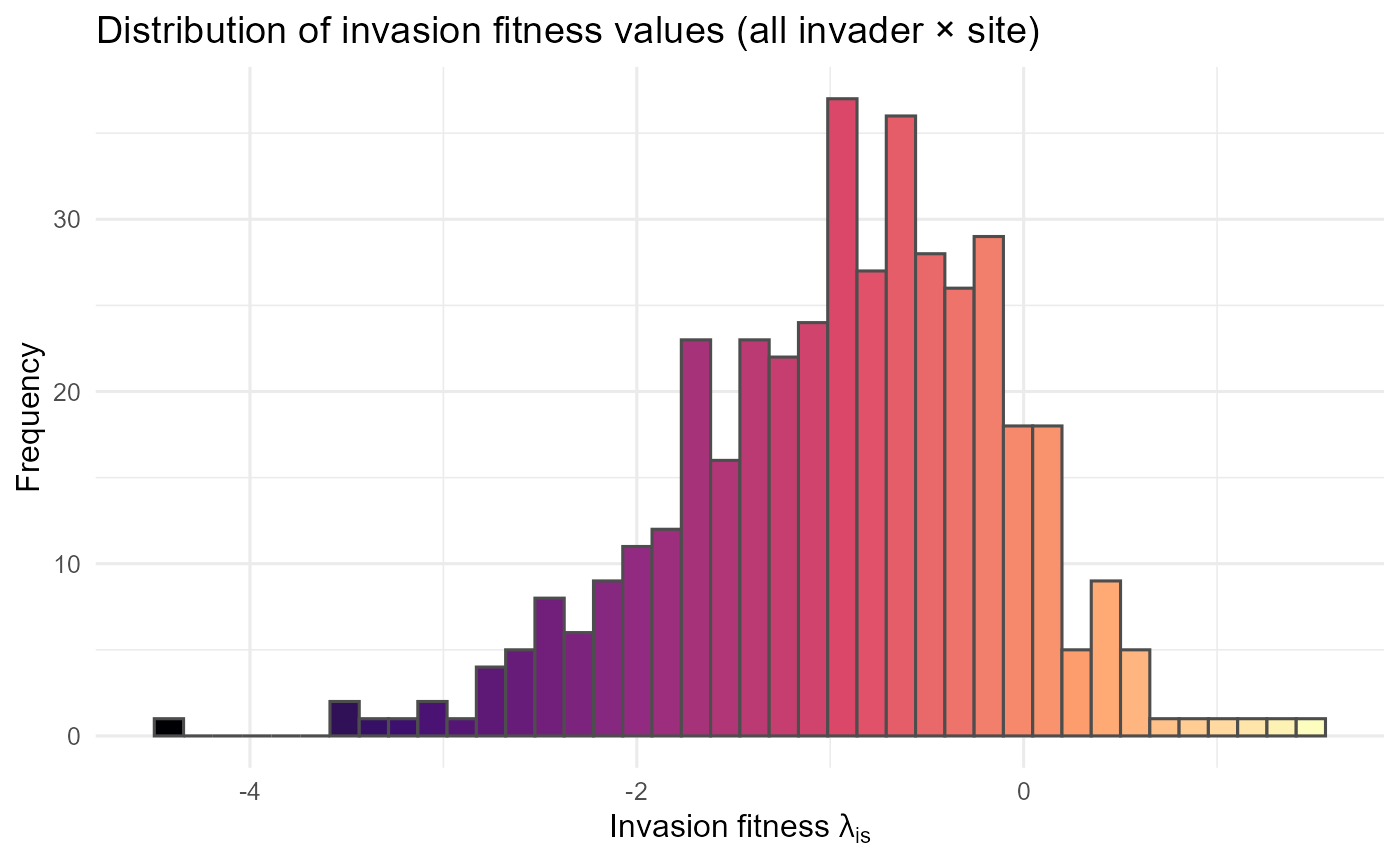

:chart_with_upwards_trend: Figure 29: The histogram shows the distribution of invasion fitness values (\(\lambda\)ᵢₛ) across all invader–site combinations. Most \(\lambda\) values fall between −3 and 0, with a strong concentration around −2, indicating that the majority of potential invasions are constrained by either abiotic conditions or biotic resistance. Only a small fraction of cases approach or exceed \(\lambda\) > 0 (to the right of the origin), highlighting that successful establishment opportunities are relatively rare. The long left tail (< −4) represents invader–site pairings where conditions are strongly unfavorable.

:bar_chart: Overall, the figure emphasizes that the invasion landscape is dominated by resistance rather than opportunity, but with occasional site–invader matches that may permit establishment. This pattern is consistent with theoretical expectations of community assembly, where most introductions fail but a minority may find niches that allow them to persist.

---

Top and bottom invaders and sites

Ranking by mean \(\lambda_{is}\) highlights consistently permissive sites and consistently risky invaders.

:bulb: Interpretation: Top invaders are candidates for vigilant monitoring; top sites are hotspots for surveillance or preventative management.

:warning: Checks/tips: Report uncertainty (e.g., bootstrapped means) when used for policy.

#> ==== Top 3 Invaders by Mean Invasion Fitness ====
#> 1. inv9: -0.388
#> 2. inv7: -0.435
#> 3. inv5: -0.864
#> 
#> ==== Bottom 3 Invaders by Mean Invasion Fitness ====
#> 1. inv1: -1.078
#> 2. inv4: -1.216
#> 3. inv8: -1.387
#> 
#> ==== Top 3 Sites by Mean Invasion Fitness ====
#> 1. 401: 1.485
#> 2. 884: 1.396
#> 3. 695: 1.136
#> 
#> ==== Bottom 3 Sites by Mean Invasion Fitness ====
#> 1. 417: -3.474
#> 2. 428: -3.523
#> 3. 558: -4.419

---

Functional correlates of invasion success

We relate invader traits to mean \(\lambda_{is}\) to identify functional profiles linked to high or low establishment.

:bulb: Interpretation: Strong positive (or negative) correlations for continuous traits, and high/low trait-level means for categorical traits, suggest mechanistic drivers worth testing experimentally.

:warning: Checks/tips: Standardise continuous traits; ensure categorical levels are well populated; treat results as exploratory unless validated.

#> ==== Top 3 Continuous Traits by Correlation with Mean Invasion Fitness ====
#> trait_cont7: 0.732
#> trait_cont2: 0.551
#> trait_cont1: 0.113
#> 
#> ==== Bottom 3 Continuous Traits by Correlation with Mean Invasion Fitness ====
#> trait_cont8: -0.427
#> trait_cont4: -0.435
#> trait_cont5: -0.449
#> ==== Categorical Traits: Top Value per Trait by Mean Invasion Fitness ====
#> trait_cat11: grassland (-0.82)
#> trait_cat12: nocturnal (-0.90)
#> trait_cat13: bivoltine (-0.88)
#> trait_cat14: nectarivore (-0.71)
#> trait_cat15: migratory (-0.92)

---

Faceted maps for key invaders

We visualise spatial patterns for the top and bottom invaders identified above to link traits, environments, and community context.

:bulb: Interpretation: Hotspots for top invaders mark priority regions; uniformly low values for bottom invaders highlight robust sites or mismatched niches.

:warning: Checks/tips: Use a centred colour scale; show boundaries for orientation; keep facet order consistent with ranks.

---

:hourglass_flowing_sand: Step-by-step in this section: 1. select invaders ➔ 2. compute z-MAD standardized fitness ➔ 3. build facet labels ordered by mean \(\lambda\) ➔ 4. map with a centered palette ➔ 5. show relative advantage vs site mean ➔ 6. optionally overlay contours (\(\lambda>0\)); top decile).

Select key invaders (top & bottom)

# Objects assumed: df_inv (site, invader, x, y, lambda), rsa (sf boundary)
# Also assumed: top3_inv, bottom3_inv with columns 'invader'

# Select key invaders
key_invaders = c(top3_inv$invader, bottom3_inv$invader) |> unique()

lambda_key = df_inv |>
  dplyr::filter(invader %in% key_invaders) |>
  dplyr::mutate(invader = factor(invader, levels = key_invaders))
dim(lambda_key)
#> [1] 2490   11

Compute z-MAD standardization of (\(\lambda\))

# z-MAD for lambda (avoid divide-by-zero)
med = median(lambda_key$lambda, na.rm = TRUE)
mad_ = mad(lambda_key$lambda, na.rm = TRUE)
if (!is.finite(mad_) || mad_ == 0) mad_ = sd(lambda_key$lambda, na.rm = TRUE)

lambda_key = lambda_key |>
  dplyr::mutate(lambda_zmad = (lambda - med) / mad_)
dim(lambda_key)
#> [1] 2490   12

Order facets by mean (\(\lambda\)) and build labels

# Order facets by mean lambda and create labels
lab_means = lambda_key |>
  dplyr::group_by(.data$invader) |>
  dplyr::summarise(mu = mean(.data$lambda, na.rm = TRUE), .groups = "drop") |>
  dplyr::arrange(dplyr::desc(.data$mu)) |>
  dplyr::mutate(label = sprintf("%s (mean \u03BB = %.2f)", .data$invader, .data$mu))

lab_levels = lab_means$label

lambda_key2 <- lambda_key |>
  dplyr::left_join(lab_means |> dplyr::select(invader, label), by = "invader", suffix = c(".x", ".y")) |>
  dplyr::mutate(label = dplyr::coalesce(label.y, label.x)) |>   # prefer joined label
  dplyr::select(-label.x, -label.y) |>
  dplyr::mutate(label = factor(label, levels = lab_levels))
names(lambda_key2)
#>  [1] "site"            "invader"         "val"             "lambda"         
#>  [5] "mode"            "x"               "y"               "val_f"          
#>  [9] "site_cluster"    "invader_cluster" "lambda_zmad"     "label"

Ordered faceted maps (centered palette)

# Load the national boundary
library(ggplot2)
rsa = sf::st_read(system.file("extdata", "rsa.shp", package = "invasimapr"))
#> Reading layer `rsa' from data source 
#>   `C:\Users\macfadyen\AppData\Local\R\win-library\4.5\invasimapr\extdata\rsa.shp' 
#>   using driver `ESRI Shapefile'
#> Simple feature collection with 11 features and 8 fields
#> Geometry type: MULTIPOLYGON
#> Dimension:     XY
#> Bounding box:  xmin: 16.45189 ymin: -34.83417 xmax: 32.94498 ymax: -22.12503
#> Geodetic CRS:  WGS 84

# Diverging palette + clearer midpoint
ggplot2::ggplot(lambda_key2, ggplot2::aes(x, y, fill = lambda_zmad)) +
  ggplot2::geom_tile() +
  ggplot2::geom_sf(data = rsa, inherit.aes = FALSE, fill = NA, color = "black", linewidth = 0.5) +
  ggplot2::facet_wrap(~ label, ncol = 3) +
  scico::scale_fill_scico(
    palette = "vik", limits = c(-4, 4), oob = scales::squish,
    name = "Lambda (z-MAD)", midpoint = 0
  ) +
  ggplot2::labs(title = "Spatial invasion fitness (facets ordered by mean \u03BB)",
       x = "Longitude", y = "Latitude") +
  theme_minimal(12) +
  theme(panel.grid = ggplot2::element_blank())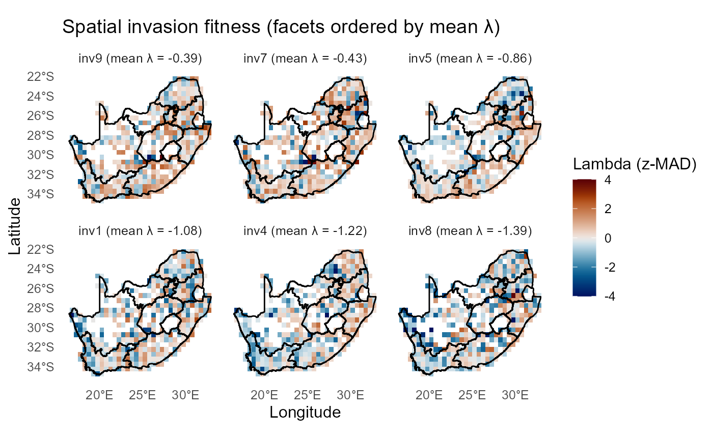

:chart_with_upwards_trend: Figure 30: This figure compares the spatial distribution of invasion fitness (\(\lambda\), expressed as z-MAD) for the three highest- and three lowest-ranked invaders, ordered by their mean \(\lambda\) values. Across invaders, spatial variation is structured by a common underlying pattern: inland and northeastern regions generally exhibit higher-than-expected invasion fitness (warm tones), whereas coastal and southwestern areas are consistently characterized by lower fitness (cool tones). The top-ranked invaders (inv5, inv9, inv10) show broader and more contiguous zones of positive \(\lambda\), indicating relatively favourable conditions across multiple regions. In contrast, the bottom-ranked invaders (inv8, inv2, inv1) display more extensive and spatially consistent negative \(\lambda\) values, with only small and fragmented pockets of opportunity.

Alternative gradient (viridis/magma)

ggplot2::ggplot(lambda_key, ggplot2::aes(x = x, y = y, fill = lambda_zmad)) +
  ggplot2::geom_tile() +
  ggplot2::geom_sf(data = rsa, inherit.aes = FALSE, fill = NA, color = "black", linewidth = 0.5) +
  ggplot2::facet_wrap(~ invader, ncol = 3) +
  ggplot2::scale_fill_gradientn(
    colours  = viridisLite::magma(256, direction = -1),
    rescaler = function(x, ...) scales::rescale_mid(x, mid = 0),
    limits   = c(-4, 4), oob = scales::squish,
    name     = "Lambda (z-MAD)"
  ) +
  labs(title = "Spatial invasion fitness for top- and bottom-ranked invaders",
       x = "Longitude", y = "Latitude") +
  theme_minimal(12) +
  theme(panel.grid = ggplot2::element_blank())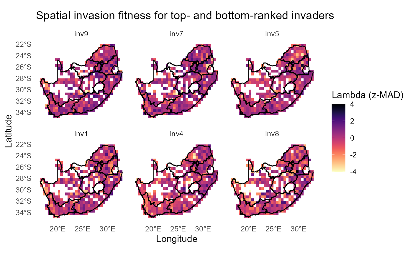

:chart_with_upwards_trend: Figure 31: Same maps with an alternative diverging look using magma centered at 0.

Invader advantage relative to site mean

# Emphasize invader-specific advantage relative to the same sites
site_means = df_inv |>
  dplyr::group_by(site) |>
  dplyr::summarise(site_mean = mean(lambda, na.rm = TRUE), .groups = "drop")

lambda_rel = lambda_key |>
  dplyr::left_join(site_means, by = "site") |>
  dplyr::mutate(delta_lambda = lambda - site_mean)

ggplot2::ggplot(lambda_rel, aes(x, y, fill = delta_lambda)) +
  ggplot2::geom_tile() +
  ggplot2::geom_sf(data = rsa, inherit.aes = FALSE, fill = NA, color = "black", linewidth = 0.5) +
  ggplot2::facet_wrap(~ invader, ncol = 3) +
  ggplot2::scale_fill_gradient2(
    name = expression(Delta * lambda),
    low = "#3b4cc0", mid = "white", high = "#b40426", midpoint = 0
  ) +
  labs(title = "Invader advantage relative to site mean (\u0394\u03BB)",
       x = "Longitude", y = "Latitude") +
  theme_minimal(12) +
  theme(panel.grid = ggplot2::element_blank())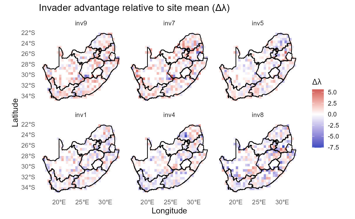

:chart_with_upwards_trend: Figure 32: Deviations from each site’s mean (\(\lambda\)) (positive = invader outperforms the typical invader at that site).

:bar_chart: Together, these contrasts highlight that invader performance is shaped by both shared environmental templates and invader-specific deviations, with higher-ranked invaders better aligned with spatial hotspots of opportunity.

:sparkles: Overall importance: This compact set—distribution, ranks, trait links, and maps—forms a practical reporting dashboard for stakeholders.

:bulb: Summary. You now have system-level summaries, interpretable ranks, functional signals, and spatial views—ready for communication and action.

:warning: Checks/tips: * Use a centered color scale so zero is visually neutral. * Keep facet order consistent (use the label factor). * If thresholds should be invader-specific, compute per-invader thr_i and draw contours per group (loop or group_split()), since breaks can’t vary within a single geom_contour() call. * For publication, export figures with fixed dimensions and fonts (e.g., ggsave(..., width=7, height=6, dpi=300)).

---

Session information

sessionInfo()
#> R version 4.5.2 (2025-10-31 ucrt)
#> Platform: x86_64-w64-mingw32/x64
#> Running under: Windows 11 x64 (build 26200)
#> 
#> Matrix products: default
#>   LAPACK version 3.12.1
#> 
#> locale:
#> [1] LC_COLLATE=English_South Africa.utf8  LC_CTYPE=English_South Africa.utf8   
#> [3] LC_MONETARY=English_South Africa.utf8 LC_NUMERIC=C                         
#> [5] LC_TIME=English_South Africa.utf8    
#> 
#> time zone: Africa/Johannesburg
#> tzcode source: internal
#> 
#> attached base packages:
#> [1] stats     graphics  grDevices utils     datasets  methods   base     
#> 
#> other attached packages:
#> [1] ggplot2_4.0.0
#> 
#> loaded via a namespace (and not attached):
#>   [1] Rdpack_2.6.5        DBI_1.2.3           gridExtra_2.3      
#>   [4] permute_0.9-8       sandwich_3.1-1      rlang_1.1.7        
#>   [7] magrittr_2.0.4      multcomp_1.4-28     otel_0.2.0         
#>  [10] matrixStats_1.5.0   e1071_1.7-16        compiler_4.5.2     
#>  [13] mgcv_1.9-3          systemfonts_1.2.3   vctrs_0.7.1        
#>  [16] stringr_1.6.0       pkgconfig_2.0.3     shape_1.4.6.1      
#>  [19] fastmap_1.2.0       backports_1.5.0     labeling_0.4.3     
#>  [22] rmarkdown_2.30      nloptr_2.2.1        ragg_1.5.0         
#>  [25] purrr_1.2.0         xfun_0.56           glmnet_4.1-10      
#>  [28] cachem_1.1.0        jsonlite_2.0.0      scico_1.5.0        
#>  [31] terra_1.8-54        broom_1.0.10        parallel_4.5.2     
#>  [34] cluster_2.1.8.1     R6_2.6.1            bslib_0.9.0        
#>  [37] stringi_1.8.7       RColorBrewer_1.1-3  car_3.1-3          
#>  [40] boot_1.3-32         jquerylib_0.1.4     numDeriv_2016.8-1.1
#>  [43] estimability_1.5.1  Rcpp_1.1.0          iterators_1.0.14   
#>  [46] knitr_1.51          zoo_1.8-14          Matrix_1.7-4       
#>  [49] splines_4.5.2       glmmTMB_1.1.11      tidyselect_1.2.1   
#>  [52] viridis_0.6.5       rstudioapi_0.17.1   abind_1.4-8        
#>  [55] yaml_2.3.12         vegan_2.7-1         invasimapr_0.1.0   
#>  [58] TMB_1.9.17          codetools_0.2-20    lattice_0.22-7     
#>  [61] tibble_3.3.1        withr_3.0.2         S7_0.2.0           
#>  [64] coda_0.19-4.1       evaluate_1.0.5      desc_1.4.3         
#>  [67] survival_3.8-3      sf_1.0-21           units_0.8-7        
#>  [70] proxy_0.4-27        pillar_1.11.1       ggpubr_0.6.2       
#>  [73] carData_3.0-5       KernSmooth_2.23-26  foreach_1.5.2      
#>  [76] reformulas_0.4.3.1  insight_1.3.1       generics_0.1.4     
#>  [79] fuzzyjoin_0.1.6.1   scales_1.4.0        minqa_1.2.8        
#>  [82] xtable_1.8-4        class_7.3-23        glue_1.8.0         
#>  [85] pheatmap_1.0.13     emmeans_2.0.1       tools_4.5.2        
#>  [88] data.table_1.18.0   lme4_1.1-37         ggsignif_0.6.4     
#>  [91] fs_1.6.6            mvtnorm_1.3-3       grid_4.5.2         
#>  [94] tidyr_1.3.1         rbibutils_2.4.1     nlme_3.1-168       
#>  [97] performance_0.15.0  Formula_1.2-5       cli_3.6.5          
#> [100] textshaping_1.0.3   viridisLite_0.4.2   dplyr_1.1.4        
#> [103] gtable_0.3.6        rstatix_0.7.3       sass_0.4.10        
#> [106] digest_0.6.37       classInt_0.4-11     ggrepel_0.9.6      
#> [109] TH.data_1.1-4       htmlwidgets_1.6.4   farver_2.1.2       
#> [112] htmltools_0.5.8.1   pkgdown_2.1.3       factoextra_1.0.7   
#> [115] lifecycle_1.0.5     MASS_7.3-65