Clustering and risk scenarios

Install and load `invasimapr` and other core packages

Install from GitHub (recommended for development) or CRAN (if available) as before.

After computing invasion fitness $\lambda_{is}$ (Sections 6-7), we can mine the $\text{invader} \times \text{site}$ surface for recurring profiles. Clustering reveals groups of invaders with similar spatial success and groups of sites with similar susceptibility, enabling practical risk categories and scenario planning.

:hourglass_flowing_sand: Step-by-step this section:

We reshape the long fitness table into a matrix $\Lambda$ with rows = invaders and columns = sites;
scale and cluster rows and columns (Ward’s method) to expose structure;
assign discrete cluster labels to invaders and sites for downstream mapping and summaries; and
visualise the joint structure with a clustered heatmap.

Hierarchical clustering of invaders and sites

We treat each invader as a vector of fitness values across sites and each site as a vector across invaders. Hierarchical clustering groups invaders into “broad-spectrum” vs. “specialists” and sites into “open” vs. “resistant” community types. We scale rows/columns to neutralise magnitude, compute Euclidean distances, and apply Ward’s linkage. The number of clusters $k$ can be chosen by silhouette/gap heuristics or fixed for interpretability.

:hourglass_flowing_sand: Step-by-step this section: 1. Build the $\lambda_{is}$ matrix ➔ 2. Clean ➔ 3. Scale rows/cols ➔ 4. Compute Euclidean distances ➔ 5. Cluster with Ward’s linkage ➔ 6. Choose ($k$) (silhouette when available; else a small default) ➔ 7. Attach cluster labels back to data.

Setup helper functions

# Optional for k selection via silhouette:
has_fviz = requireNamespace("factoextra", quietly = TRUE)

# Helpers --------------------------------------------------------------
safe_scale = function(M) {
  if (is.null(dim(M))) return(matrix(M, nrow = 1L))
  sds = apply(M, 2, sd, na.rm = TRUE)
  z = scale(M, center = TRUE, scale = sds)
  z[is.na(z)] = 0  # handles sd=0 columns
  z
}

safe_kmax = function(X, kmax = 10L) {
  n = nrow(X); if (is.null(n) || n < 3L) return(NA_integer_)
  min(kmax, n - 1L)  # k in [2, n-1]
}

choose_k_silhouette = function(X, kmax = 10L, nstart = 25L) {
  kmax_safe = safe_kmax(X, kmax)
  if (is.na(kmax_safe) || !has_fviz) return(NA_integer_)
  gg = factoextra::fviz_nbclust(
    as.data.frame(X), FUNcluster = kmeans, method = "silhouette",
    k.max = kmax_safe, nstart = nstart
  )
  d = gg$data
  if (!is.null(d) && all(c("clusters","y") %in% names(d))) d$clusters[which.max(d$y)] else NA_integer_
}

Assemble the invader × site fitness matrix ($\lambda$)

We pivot long results (one row per site×invader) to a wide matrix with rows = invaders, cols = sites. If multiple draws exist, we take the mean per cell. Then drop rows/columns that are entirely NA (or all missing after earlier filters). If too few remain, we bail out gracefully.

lambda_mat = fit$summary$establish_long |>
  dplyr::select(invader, site, lambda) |>
  tidyr::pivot_wider(
    id_cols = invader,
    names_from = site,
    values_from = lambda,
    values_fill = 0,
    values_fn = list(lambda = ~ mean(.x, na.rm = TRUE))
  ) |>
  tibble::column_to_rownames("invader") |>
  as.matrix()

dim(lambda_mat)     # rows=invaders, cols=sites
#> [1]  10 415

lambda_mat_noNA = lambda_mat[
  rowSums(is.na(lambda_mat)) < ncol(lambda_mat),
  colSums(is.na(lambda_mat)) < nrow(lambda_mat),
  drop = FALSE
]

if (nrow(lambda_mat_noNA) < 2L || ncol(lambda_mat_noNA) < 2L) {
  warning("Too few invaders or sites for clustering; assigning NA clusters.")
}
dim(lambda_mat_noNA)     # rows=invaders, cols=sites
#> [1]  10 415

Cluster sites (columns as observations)

We scale invader dimensions (columns) to neutralize magnitude and cluster sites via Ward.D2.

if (nrow(lambda_mat_noNA) >= 2L && ncol(lambda_mat_noNA) >= 2L) {

  X_sites = t(safe_scale(lambda_mat_noNA))  # rows = sites, cols = invaders
  keep_sites = apply(X_sites, 1, sd) > 0
  if (any(!keep_sites)) X_sites = X_sites[keep_sites, , drop = FALSE]

  site_dist  = dist(X_sites)
  site_clust = hclust(site_dist, method = "ward.D2")

  k_sites = choose_k_silhouette(X_sites, kmax = 10L)
  if (is.na(k_sites)) k_sites = max(2L, min(5L, nrow(X_sites)))

  site_groups_ok = cutree(site_clust, k = k_sites)  # named vector (kept sites)

  # Reinsert dropped sites (if any) as NA; preserve original site order
  site_groups = setNames(rep(NA_integer_, ncol(lambda_mat_noNA)),
                          colnames(lambda_mat_noNA))
  site_groups[names(site_groups_ok)] = site_groups_ok
}

Cluster invaders (rows as observations)

Same idea, now with rows (invaders) as observations.

if (nrow(lambda_mat_noNA) >= 2L && ncol(lambda_mat_noNA) >= 2L) {

  X_inv = safe_scale(lambda_mat_noNA)       # rows = invaders, cols = sites
  keep_inv = apply(X_inv, 1, sd) > 0
  if (any(!keep_inv)) X_inv = X_inv[keep_inv, , drop = FALSE]

  inv_dist  = dist(X_inv)
  inv_clust = hclust(inv_dist, method = "ward.D2")

  k_inv = choose_k_silhouette(X_inv, kmax = 10L)
  if (is.na(k_inv)) k_inv = max(2L, min(5L, nrow(X_inv)))

  inv_groups_ok = cutree(inv_clust, k = k_inv)  # named vector (kept invaders)

  inv_groups = setNames(rep(NA_integer_, nrow(lambda_mat_noNA)),
                         rownames(lambda_mat_noNA))
  inv_groups[names(inv_groups_ok)] = inv_groups_ok
}

Attach cluster labels for downstream use

We create (or update) a df_inv table with one row per (site, invader) and two factor columns: site_cluster, invader_cluster. Any dropped entities become NA.

# Ensure df_inv exists
if (!exists("df_inv")) {
  df_inv = fit$summary$establish_long |>
    dplyr::select(site, invader) |>
    dplyr::distinct() |>
    dplyr::mutate(across(c(site, invader), as.character))
}

# Sanity checks: names should align with the clustered matrix
if (!all(df_inv$site %in% names(site_groups))) {
  warning("Some sites in df_inv not present in clustered matrix; setting NA.")
}
if (!all(df_inv$invader %in% names(inv_groups))) {
  warning("Some invaders in df_inv not present in clustered matrix; setting NA.")
}

df_inv = df_inv |>
  dplyr::mutate(
    site_cluster    = factor(site_groups[site],
                             levels = sort(unique(site_groups))),
    invader_cluster = factor(inv_groups[invader],
                             levels = sort(unique(inv_groups)))
  )

head(df_inv)
#> # A tibble: 6 × 11
#>   site  invader   val lambda mode          label      x     y val_f site_cluster
#>   <chr> <chr>   <int>  <dbl> <chr>         <chr>  <dbl> <dbl> <fct> <fct>       
#> 1 82    inv1        0 -1.92  probabilistic proba…  19.2 -34.8 0     1           
#> 2 83    inv1        0 -5.18  probabilistic proba…  19.8 -34.8 0     1           
#> 3 84    inv1        0 -1.21  probabilistic proba…  20.2 -34.8 0     2           
#> 4 117   inv1        1  0.220 probabilistic proba…  18.2 -34.3 1     2           
#> 5 118   inv1        0 -1.28  probabilistic proba…  18.8 -34.3 0     2           
#> 6 119   inv1        0 -1.45  probabilistic proba…  19.2 -34.3 0     1           
#> # ℹ 1 more variable: invader_cluster <fct>

:information_source: Why this matters: Cluster labels compress thousands of $\lambda_{is}$ cells into a handful of profiles that managers and analysts can reason about.

:warning: Checks/tips: * Remove rows/cols with only NA before clustering; clustering needs variation. * Scaling neutralizes magnitude so distance reflects shape of response. * If silhouette selection isn’t available, we default to a small ($k$) (2–5) for interpretability. * Store site_cluster and invader_cluster on your canonical tables for downstream stratified summaries, e.g. site-type vs invader-type risk maps.

Quick diagnostic plots

:bar_chart: Clustered $\lambda$ heatmap summarizes the joint structure of invasion fitness ($\lambda$) across invaders (rows) and sites (columns).

# Sites dendrogram
if (exists("site_clust")) plot(site_clust, main = "Sites (Ward.D2)", xlab = "", sub = "")

Site dendrogram

# Invaders dendrogram
if (exists("inv_clust")) plot(inv_clust, main = "Invaders (Ward.D2)", xlab = "", sub = "")

Invader dendrogram

:chart_with_upwards_trend: Figure 24: Dendrograms, useful to eyeball structure and plausibility (k).

# Clustered heatmap: joint structure in $\lambda$ (invader × site)
pheatmap::pheatmap(
  lambda_mat_noNA,
  kmeans_k = 5,
  color = rev(viridis::viridis(50, option = "magma", direction = 1)),
  clustering_distance_rows = "euclidean",
  clustering_distance_cols = "euclidean",
  clustering_method        = "ward.D",
  fontsize_row = 8, fontsize_col = 8,
  main = "Clustered Invasion Fitness Matrix (Invader × Site)",
  angle_col = 45
)

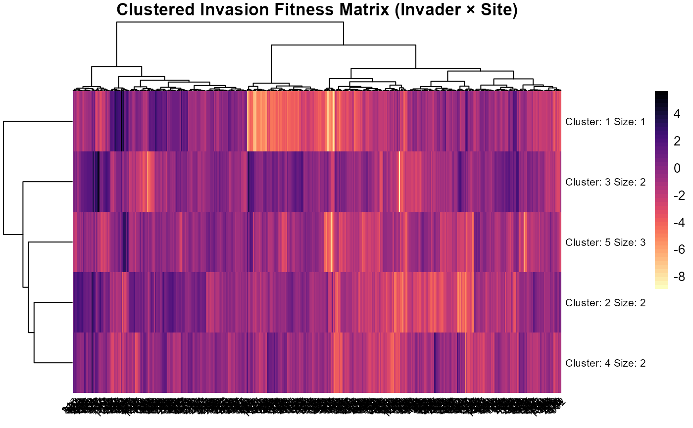
Clustered heatmap of invasion fitness

:chart_with_upwards_trend: Figure 25: The clustered heatmap summarizes the joint structure of invasion fitness ($\lambda$) across invaders (rows) and sites (columns): Colors encode $\lambda$ (yellow/white = higher fitness; purple/black = lower), and the dendrograms group invaders and sites by similarity in their $\lambda$ profiles (Ward clustering). Clear vertical bands of warmer colors indicate that site identity explains much of the variation, certain site clusters consistently offer higher fitness across many invaders, whereas horizontal blocks are weaker, implying more modest between-invader differences. The k-means split (k = 5) on the columns highlights a few distinct site regimes that alternate between high and low $\lambda$, producing contiguous stripes rather than scattered pixels. Some invader clusters show uniformly poor performance (cool rows) with only small pockets of opportunity, while others have broader tolerance with multiple site clusters showing elevated $\lambda$. Overall, the figure reveals strong spatial structure in establishment potential, with invader effects present but secondary to site-level context.

:sparkles: Overall importance: Clustering turns a dense prediction surface into a concise vocabulary of profiles for communication and planning.

:bulb: Summary. You now have invader and site cluster labels that can be mapped, ranked, and cross-tabulated with traits and environments.

Mapping site-level risk categories

To support spatial decisions, we translate site clusters into ordered risk categories (very-high → very-low) using mean $\lambda_{is}$ within each cluster, optionally constraining clusters to be geographically cohesive. In this section:

We use ClustGeo to blend similarity in $\Lambda$ profiles with geographic distance,
choose $k$ clusters, and then
relabel clusters by their mean site fitness into intuitive risk categories.
Finally, we map categories over the study region.

:information_source: Why this matters: The map highlights where openness to invasion concentrates and provides a stable spatial unit for monitoring and intervention.

:warning: Checks/tips: Ensure coordinate joins are correct; test a few $\alpha$ weights (0 = spatial only, 1 = fitness only); order categories by mean fitness for consistent legends.

:hourglass_flowing_sand: Step-by-step: 1. Assemble $\lambda$ ➔ 2. Prepare site coordinates ➔ 3. Build profile and spatial distances ➔ 4. Cluster with ClustGeo ➔ 5. Choose $k$ ➔ 6. Relabel clusters by mean $\lambda$ ➔ 7. Map

Setup (packages, inputs)

# Optional: spatial / clustering helpers
has_sf      = requireNamespace("sf", quietly = TRUE)
has_clgeo   = requireNamespace("ClustGeo", quietly = TRUE)

# Expected objects:
# - fit$summary$establish_long or fit$fitness$lambda_long with (site, invader, lambda)
# - fitness_df with site-level summaries incl. site coords (x,y) or an sf geometry
# - rsa (optional sf boundary for context)

Assemble a long table of ($\lambda$) (one row per site × invader)

Guard against duplicates by averaging within (site, invader) and drop fully-NA rows/columns for stability.

lambda_long = if (!is.null(fit$fitness$lambda_long)) {
  fit$fitness$lambda_long
} else {
  fit$summary$establish_long
}

lambda_mean = lambda_long |>
  dplyr::select(site, invader, lambda) |>
  dplyr::mutate(across(c(site, invader), as.character)) |>
  dplyr::group_by(site, invader) |>
  dplyr::summarise(mean_lambda = mean(lambda, na.rm = TRUE), .groups = "drop")

# Drop fully-NA rows/columns for stability
lambda_mat = lambda_mean |>
  tidyr::pivot_wider(
    id_cols = invader, names_from = site, values_from = mean_lambda,
    values_fill = 0, values_fn = list(mean_lambda = ~ mean(.x, na.rm = TRUE))
  ) |>
  tibble::column_to_rownames("invader") |>
  as.matrix()
dim(lambda_mat)
#> [1]  10 415

lambda_mat_noNA = lambda_mat[
  rowSums(is.na(lambda_mat)) < ncol(lambda_mat),
  colSums(is.na(lambda_mat)) < nrow(lambda_mat),
  drop = FALSE
]

stopifnot(ncol(lambda_mat_noNA) >= 2L, nrow(lambda_mat_noNA) >= 2L)
dim(lambda_mat_noNA)
#> [1]  10 415

Prepare site coordinates (x,y)

Accepts fitness_df either with numeric x,y columns or as sf with point geometry.

# Extract site ids to be clustered (columns of lambda_mat_noNA)
site_ids = colnames(lambda_mat_noNA)

# Get coordinates for these sites
if (has_sf && inherits(fitness_df, "sf")) {
  # If sf, derive lon/lat (or projected) from geometry
  xy = sf::st_coordinates(sf::st_centroid(fitness_df))
  coords_df = cbind(st_drop_geometry(fitness_df), x = xy[,1], y = xy[,2])
} else {
  coords_df = fitness_df
}

stopifnot(all(c("site","x","y") %in% names(coords_df)))
site_coords = coords_df |>
  dplyr::mutate(site = as.character(site)) |>
  dplyr::filter(site %in% site_ids) |>
  dplyr::select(site, x, y)

# Reorder to match site_ids; keep only complete cases
site_coords = site_coords[match(site_ids, site_coords$site), ]
ok = stats::complete.cases(site_coords$x, site_coords$y)
stopifnot(any(ok))  # need at least some sites with coords

Build distances: profile (D1) + geographic (D0)

Scale site profiles (rows) to neutralize magnitude; then compute Euclidean distances.

# X = sites × invaders (scaled across invaders)
scale_cols = function(M) {
  sds = apply(M, 2, sd, na.rm = TRUE)
  Z   = scale(M, center = TRUE, scale = sds); Z[is.na(Z)] = 0; Z
}

X  = scale_cols(t(lambda_mat_noNA[, ok, drop = FALSE]))  # rows = sites(ok)
D1 = dist(X)                                            # profile distance

D0 = dist(as.matrix(site_coords$x[ok]) |> cbind(site_coords$y[ok]))
# Equivalent: dist(cbind(site_coords$x[ok], site_coords$y[ok]))

Run ClustGeo (blend profile + spatial cohesion)

Tune ($\alpha \in$ [0,1]): 0 = spatial only; 1 = profile only. (Optional) try a few ($\alpha$) values and inspect inertia to pick a trade-off.

if (!has_clgeo) stop("ClustGeo not installed. install.packages('ClustGeo')")

alpha = 0.3   # adjust: higher = prioritize lambda profiles; lower = more spatial cohesion
tree  = ClustGeo::hclustgeo(D0, D1, alpha = alpha)

# Choose k (fixed or heuristic). For spatial categories, a small k is typical.
k = 5
site_groups_ok = stats::cutree(tree, k = k)  # names are sites with ok coords

# Reinsert NAs for sites lacking coords; order = site_ids
site_groups = setNames(rep(NA_integer_, length(site_ids)), site_ids)
site_groups[names(site_groups_ok)] = site_groups_ok

Optional: alpha tuning curve

# Within-cluster sum of squares from a distance matrix
# Works for Euclidean distances (e.g., dist() on scaled data or coordinates).
# W(C) = 0.5 / n_C * sum_{i,j in C} d(i,j)^2  ;  W = sum_C W(C)

withinss_dist = function(D, groups) {
  if (inherits(D, "dist")) D = as.matrix(D)
  g = as.factor(groups)
  idx = split(seq_len(nrow(D)), g)
  w = vapply(idx, function(I) {
    n = length(I)
    if (n <= 1L) return(0)
    Dij2 = D[I, I, drop = FALSE]^2
    sum(Dij2) / (2 * n)
  }, numeric(1))
  sum(w)
}

# Total sum of squares from a distance matrix: T = 0.5/n * sum_{i,j} d(i,j)^2
totss_dist = function(D) {
  if (inherits(D, "dist")) D = as.matrix(D)
  n = nrow(D)
  if (n <= 1L) return(0)
  sum(D^2) / (2 * n)
}

# Evaluate a grid of alpha to visualize within-cluster inertia trade-off
alphas = seq(0, 1, by = 0.1)

# Precompute totals for normalization (optional)
T1 = totss_dist(D1)   # profile total inertia
T0 = totss_dist(D0)   # spatial total inertia

alpha_curve = lapply(alphas, function(a) {
  tr = ClustGeo::hclustgeo(D0, D1, alpha = a)
  gr = cutree(tr, k = k)

  W1 = withinss_dist(D1, gr)         # within-cluster profile inertia
  W0 = withinss_dist(D0, gr)         # within-cluster spatial inertia
  data.frame(alpha = a,
             W1 = W1,  W1_rel = if (T1 > 0) W1/T1 else NA_real_,
             W0 = W0,  W0_rel = if (T0 > 0) W0/T0 else NA_real_)
})
alpha_curve = do.call(rbind, alpha_curve)

# Plot (relative values 0–1 are easiest to compare)
ggplot2::ggplot(alpha_curve, ggplot2::aes(alpha)) +
  ggplot2::geom_line(ggplot2::aes(y = W1_rel), linewidth = 0.8) +
  ggplot2::geom_point(ggplot2::aes(y = W1_rel), size = 1.2) +
  ggplot2::geom_line(ggplot2::aes(y = W0_rel), linetype = 2) +
  ggplot2::geom_point(ggplot2::aes(y = W0_rel), size = 1.2, shape = 1) +
  ggplot2::labs(y = "Relative within-cluster inertia",
       title = "Alpha trade-off: profile (solid) vs spatial (dashed)",
       subtitle = paste("k =", k)) +
  ggplot2::theme_minimal(11)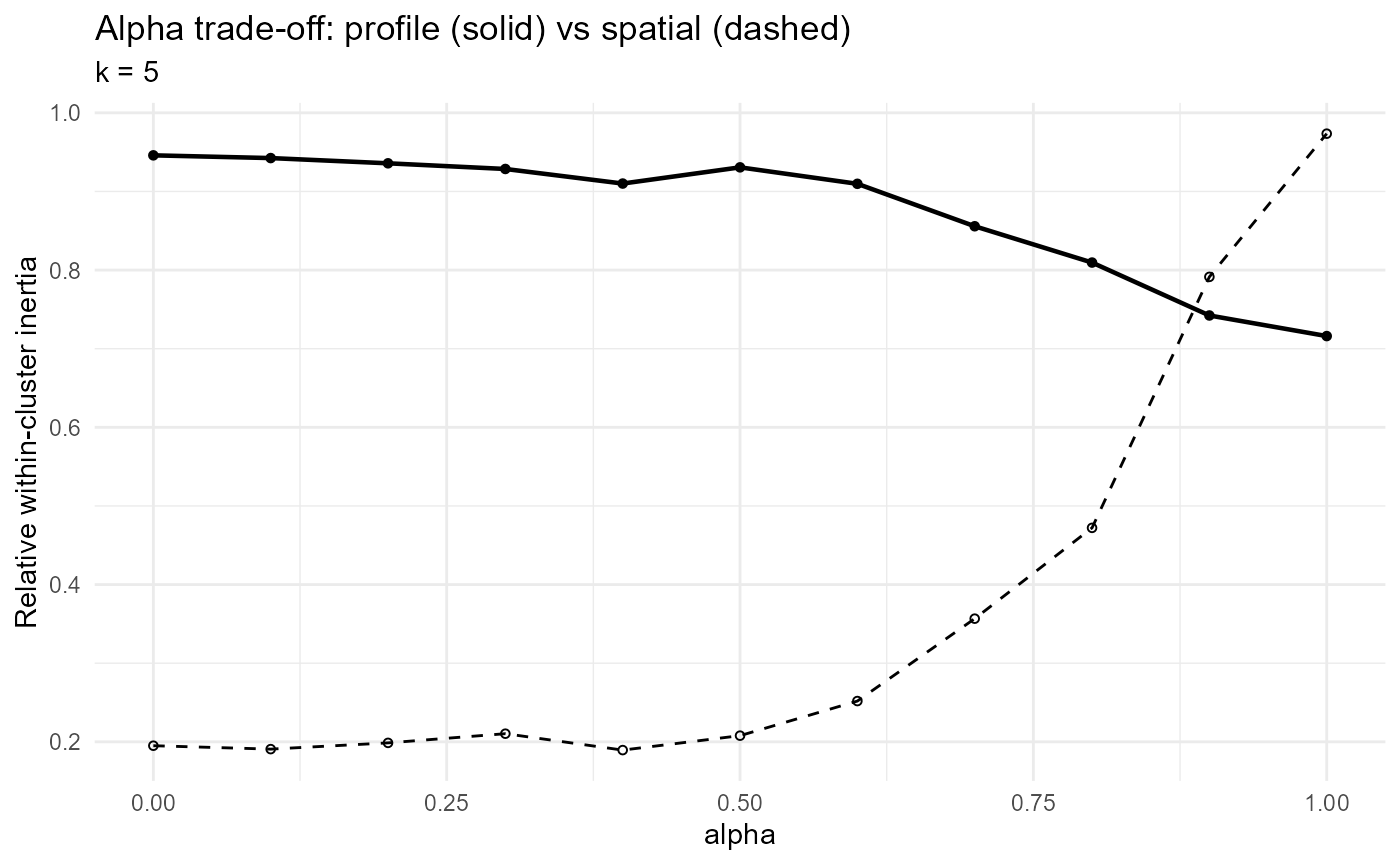

Effect of `ClustGeo` mixing parameter ($lpha$) on cluster compactness

:chart_with_upwards_trend: Figure 26: Trade-off curve showing how the choice of the ClustGeo mixing parameter ($\alpha$) affects clustering compactness in trait-profile space (solid line) versus geographic space (dashed line). At ($\alpha=0$), clusters are maximally cohesive geographically but poorly capture profile similarity; at ($\alpha=1$), the reverse holds. The curve suggests that intermediate values ($(\alpha \approx 0.3!-!0.6)$) provide a reasonable balance, with modest loss of profile compactness but large gains in spatial cohesion.

Order clusters by mean site fitness → ordered risk categories

Compute a site-level mean ($\lambda$); order clusters by descending mean; map to labels.

# Site-level mean lambda
site_lambda_mean = lambda_mean |>
  dplyr::group_by(site) |>
  dplyr::summarise(lambda_mean = mean(mean_lambda, na.rm = TRUE), .groups = "drop")

# Rank clusters by mean site lambda
tmp = data.frame(site = names(site_groups), cluster = site_groups) |>
  dplyr::left_join(site_lambda_mean, by = "site") |>
  dplyr::group_by(cluster) |>
  dplyr::summarise(mu = mean(lambda_mean, na.rm = TRUE), .groups = "drop") |>
  dplyr::arrange(desc(mu))

risk_labels = c("very-high","high","medium","low","very-low")[seq_len(nrow(tmp))]
remap = setNames(risk_labels, tmp$cluster)

# Final site table with ordered categories
site_sum = site_coords |>
  dplyr::transmute(site, x, y,
            site_cluster = remap[as.character(site_groups[site])],
            site_category = factor(site_cluster, levels = risk_labels))

Map the categories

Use either a gridded backdrop or your sf boundary. If fitness_df is gridded, tiles work; if polygons, join on site and plot geometry.

p = ggplot2::ggplot(site_sum, ggplot2::aes(x = x, y = y, fill = site_category)) +
  ggplot2::geom_tile(color = NA) +
  ggplot2::labs(title = "Spatial invasion risk (ClustGeo-constrained categories)",
       x = "Longitude", y = "Latitude", fill = "Site invasibility") +
  ggplot2::scale_fill_brewer(palette = "RdYlBu", direction = 1, drop = FALSE) +
  ggplot2::theme_minimal(12) +
  ggplot2::theme(panel.grid = ggplot2::element_blank(),
        legend.position = "right")

# Add boundary if available
if (exists("rsa") && has_sf && inherits(rsa, "sf")) {
  p = p + ggplot2::geom_sf(data = rsa, inherit.aes = FALSE, fill = NA, color = "black", size = 0.5)
}
p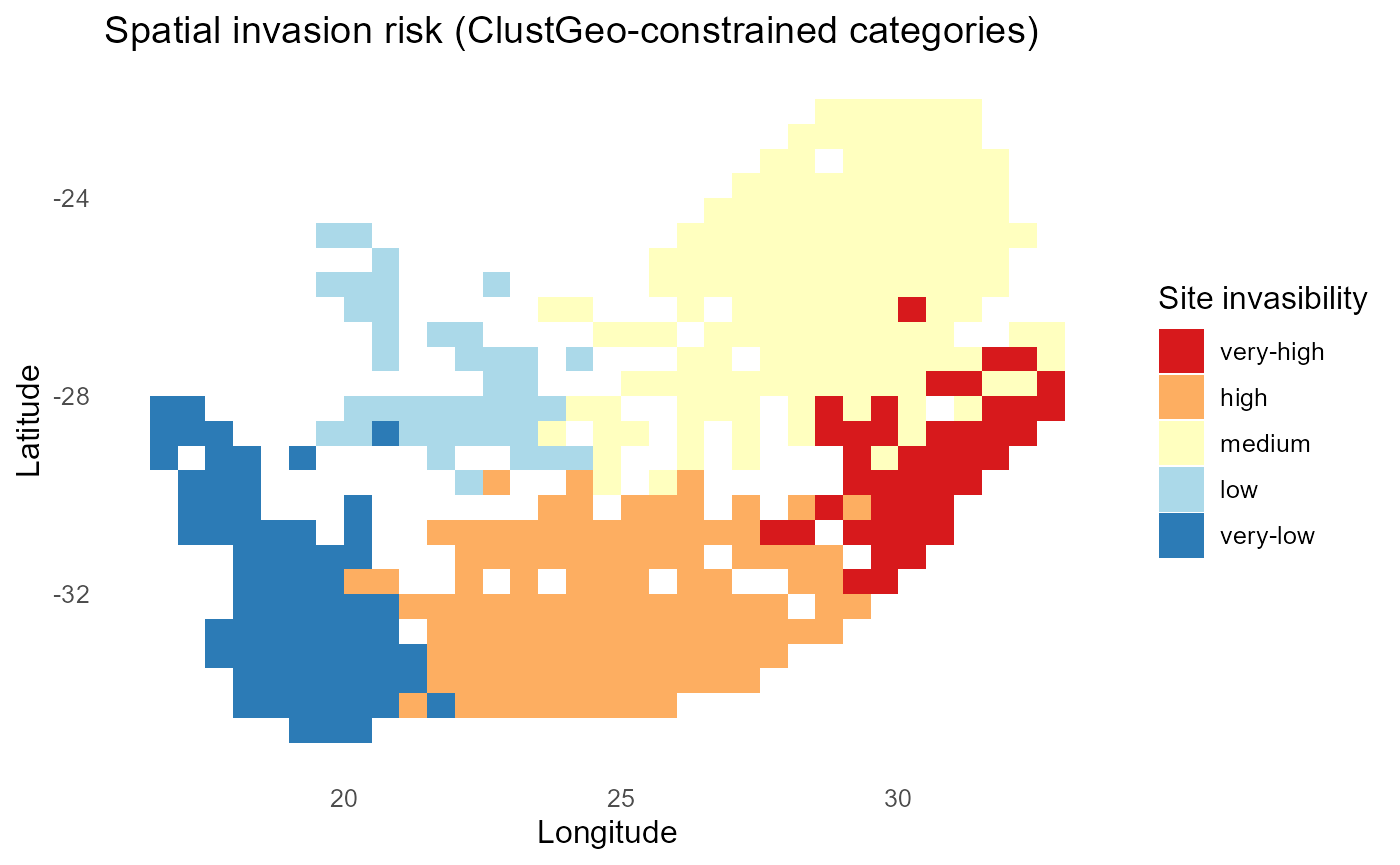

Spatial categories of invasion risk

:chart_with_upwards_trend: Figure 27: The map depicts spatial categories of invasion risk derived from a ClustGeo clustering that jointly considers site-level invasion fitness ($\lambda$ profiles across invaders) and geographic proximity. Each grid cell is assigned to one of five ordered categories, very high, high, medium, low, and very low invasibility, based on the mean establishment potential of invaders at that location.

:bar_chart: Two patterns emerge: First, invasion risk is spatially structured, with contiguous clusters of high-risk sites (red) concentrated in the southern and central regions, and very-high categories also evident in the northeast. These regions combine favorable abiotic conditions with invader-compatible resident communities. Second, low and very-low risk sites (blue shades) form coherent zones, often in the western and coastal areas, suggesting environmental filtering or strong resident resistance. Because the categories are constrained by geography, the map highlights regional-scale patterns rather than isolated hotspots. This makes it useful for decision-making, since it aligns biological risk signals with practical spatial units for monitoring and intervention. In short, the figure reveals where invasion pressure is expected to be greatest, where resistance is likely strongest, and how these patterns are distributed across the South African landscape.

Cluster-wise summaries for reporting

Summarize mean/SD/CV of ($\lambda$) by risk category, and across (site × invader) cells.

lambda_with_cat = lambda_mean |>
  dplyr::left_join(dplyr::select(site_sum, site, site_category), by = "site")

summ_sitecat = lambda_with_cat |>
  dplyr::group_by(site_category) |>
  dplyr::summarise(
    n_cells = dplyr::n(),
    mean_lambda = mean(mean_lambda, na.rm = TRUE),
    sd_lambda   = sd(mean_lambda, na.rm = TRUE),
    cv_lambda   = sd_lambda / mean_lambda,
    q10 = quantile(mean_lambda, 0.10, na.rm = TRUE),
    q50 = quantile(mean_lambda, 0.50, na.rm = TRUE),
    q90 = quantile(mean_lambda, 0.90, na.rm = TRUE),
    .groups = "drop"
  )

summ_sitecat
#> # A tibble: 5 × 8
#>   site_category n_cells mean_lambda sd_lambda cv_lambda    q10    q50    q90
#>   <fct>           <int>       <dbl>     <dbl>     <dbl>  <dbl>  <dbl>  <dbl>
#> 1 very-high         420      -0.107        NA        NA -0.107 -0.107 -0.107
#> 2 high             1120      -0.743        NA        NA -0.743 -0.743 -0.743
#> 3 medium           1520      -0.910        NA        NA -0.910 -0.910 -0.910
#> 4 low               390      -1.23         NA        NA -1.23  -1.23  -1.23 
#> 5 very-low          700      -1.60         NA        NA -1.60  -1.60  -1.60

Quick barplot of category means:

ggplot2::ggplot(summ_sitecat,
       ggplot2::aes(x = site_category, y = mean_lambda, fill = site_category)) +
  ggplot2::geom_col(show.legend = FALSE) +
  ggplot2::geom_errorbar(ggplot2::aes(ymin = mean_lambda - 1.96*sd_lambda/sqrt(n_cells),
                    ymax = mean_lambda + 1.96*sd_lambda/sqrt(n_cells)),
                width = 0.15) +
  ggplot2::labs(x = "Risk category", y = expression("Mean " * lambda),
       title = expression("Category-wise summaries of " * lambda)) +
  ggplot2::theme_minimal(11)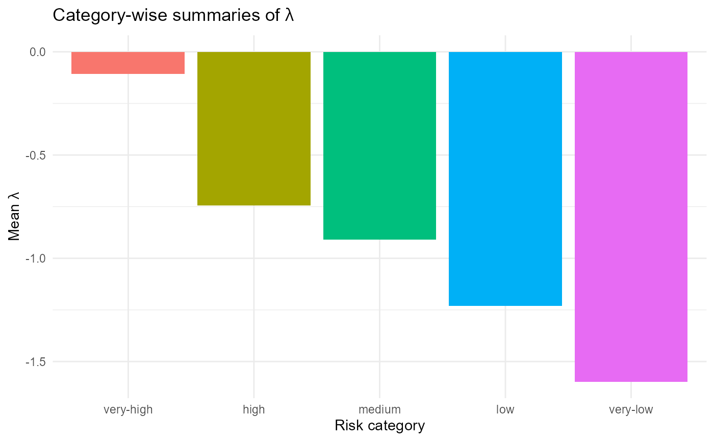

Mean invasion fitness

:chart_with_upwards_trend: Figure 28: Category-wise mean invasion fitness ($\lambda$) across ordered site risk categories (very-high to very-low). Sites assigned to the very-high category exhibit near-zero or slightly positive mean fitness values, indicating conditions most favorable to invader establishment. In contrast, low and very-low categories show strongly negative mean fitness, reflecting resistant community conditions. The monotonic decline confirms that the clustering and relabeling successfully captured a gradient of invasion risk.

:sparkles: Overall importance: Clustering + mapping yields actionable spatial units and invader types for prioritising surveillance and control.

:bulb: Summary. You now have spatially coherent site categories and interpretable invader categories that align with the full fitness surface.

:warning: Checks/tips: * Coordinates: confirm site ↔︎ coord join; if using sf, verify CRS. * Alpha: test a few ($\alpha$) (e.g., 0, 0.3, 0.6, 1) and inspect inertia to trade off cohesion vs profile similarity. * k: small ($k$) (3-6) aids communication; fix ($k$) for comparability across runs. * Ordering: always order labels by descending mean ($\lambda$) to keep legends consistent. * Missing coords: sites without coordinates get NA clusters; handle explicitly if mapping is required.

Session information

sessionInfo()
#> R version 4.5.2 (2025-10-31 ucrt)
#> Platform: x86_64-w64-mingw32/x64
#> Running under: Windows 11 x64 (build 26200)
#> 
#> Matrix products: default
#>   LAPACK version 3.12.1
#> 
#> locale:
#> [1] LC_COLLATE=English_South Africa.utf8  LC_CTYPE=English_South Africa.utf8   
#> [3] LC_MONETARY=English_South Africa.utf8 LC_NUMERIC=C                         
#> [5] LC_TIME=English_South Africa.utf8    
#> 
#> time zone: Africa/Johannesburg
#> tzcode source: internal
#> 
#> attached base packages:
#> [1] stats     graphics  grDevices utils     datasets  methods   base     
#> 
#> loaded via a namespace (and not attached):
#>   [1] Rdpack_2.6.5        DBI_1.2.3           gridExtra_2.3      
#>   [4] permute_0.9-8       sandwich_3.1-1      rlang_1.1.7        
#>   [7] magrittr_2.0.4      multcomp_1.4-28     otel_0.2.0         
#>  [10] matrixStats_1.5.0   e1071_1.7-16        compiler_4.5.2     
#>  [13] mgcv_1.9-3          systemfonts_1.2.3   vctrs_0.7.1        
#>  [16] stringr_1.6.0       pkgconfig_2.0.3     shape_1.4.6.1      
#>  [19] fastmap_1.2.0       backports_1.5.0     labeling_0.4.3     
#>  [22] utf8_1.2.6          rmarkdown_2.30      nloptr_2.2.1       
#>  [25] ragg_1.5.0          purrr_1.2.0         xfun_0.56          
#>  [28] glmnet_4.1-10       cachem_1.1.0        ClustGeo_2.1       
#>  [31] jsonlite_2.0.0      terra_1.8-54        broom_1.0.10       
#>  [34] parallel_4.5.2      cluster_2.1.8.1     R6_2.6.1           
#>  [37] bslib_0.9.0         stringi_1.8.7       RColorBrewer_1.1-3 
#>  [40] car_3.1-3           boot_1.3-32         jquerylib_0.1.4    
#>  [43] numDeriv_2016.8-1.1 estimability_1.5.1  Rcpp_1.1.0         
#>  [46] iterators_1.0.14    knitr_1.51          zoo_1.8-14         
#>  [49] Matrix_1.7-4        splines_4.5.2       glmmTMB_1.1.11     
#>  [52] tidyselect_1.2.1    viridis_0.6.5       rstudioapi_0.17.1  
#>  [55] abind_1.4-8         yaml_2.3.12         vegan_2.7-1        
#>  [58] invasimapr_0.1.0    TMB_1.9.17          codetools_0.2-20   
#>  [61] lattice_0.22-7      tibble_3.3.1        withr_3.0.2        
#>  [64] S7_0.2.0            coda_0.19-4.1       evaluate_1.0.5     
#>  [67] desc_1.4.3          survival_3.8-3      sf_1.0-21          
#>  [70] units_0.8-7         proxy_0.4-27        pillar_1.11.1      
#>  [73] ggpubr_0.6.2        carData_3.0-5       KernSmooth_2.23-26 
#>  [76] foreach_1.5.2       reformulas_0.4.3.1  insight_1.3.1      
#>  [79] generics_0.1.4      ggplot2_4.0.0       fuzzyjoin_0.1.6.1  
#>  [82] scales_1.4.0        minqa_1.2.8         xtable_1.8-4       
#>  [85] class_7.3-23        glue_1.8.0          pheatmap_1.0.13    
#>  [88] emmeans_2.0.1       tools_4.5.2         data.table_1.18.0  
#>  [91] lme4_1.1-37         ggsignif_0.6.4      fs_1.6.6           
#>  [94] mvtnorm_1.3-3       grid_4.5.2          tidyr_1.3.1        
#>  [97] rbibutils_2.4.1     nlme_3.1-168        performance_0.15.0 
#> [100] Formula_1.2-5       cli_3.6.5           textshaping_1.0.3  
#> [103] viridisLite_0.4.2   dplyr_1.1.4         gtable_0.3.6       
#> [106] rstatix_0.7.3       sass_0.4.10         digest_0.6.37      
#> [109] classInt_0.4-11     ggrepel_0.9.6       TH.data_1.1-4      
#> [112] htmlwidgets_1.6.4   farver_2.1.2        htmltools_0.5.8.1  
#> [115] pkgdown_2.1.3       factoextra_1.0.7    lifecycle_1.0.5    
#> [118] MASS_7.3-65

Clustering and risk scenarios

Install and load `invasimapr` and other core packages