Introduction

`invasimapr`

A novel framework to visualise trait dispersion and assess species invasiveness and site invasibility

Biological invasions are a major driver of biodiversity loss. Invasive alien species (IAS) can spread quickly, alter ecosystem processes, and displace native taxa. Because invasion outcomes depend jointly on functional traits, resident communities, and local environments, ad-hoc analyses are not enough. We need a transparent, reproducible way to quantify establishment potential at specific sites and to compare that potential across species and landscapes. invasimapr fills this gap. It is a trait-based, site-specific R package that estimates invasion fitness for candidate invaders, assembles the resident community context that constrains establishment, and turns these quantities into mappable indicators for decision making. The workflow links three pillars:

Functional trait space, which governs competitive overlap.
Environmental suitability, which determines how well species perform at a site.
Biotic competition, which reduces the chance of establishment.

Implemented in invasimapr, our framework fits a single trait-environment model and reuses it to quantify both invader performance and the resident context, ensuring internal consistency and transparent assumptions. It builds on standard tools (GLMM/GAM; Gower trait distances), yields reproducible workflows, and reports two headline metrics: site invasibility (openness of sites to newcomers) and species invasiveness (propensity of species to establish across sites). These metrics support core applications: risk assessment (flag species-trait combinations with high-establishment potential), biodiversity conservation (pinpoint vulnerable regions in trait and geographic space), and ecosystem management (anticipate community reconfiguration under invasion pressure). We synthesize results in the network invasibility cube, which organises invasion fitness across sites, species, and traits.

Network Invasibility Cube

The network invasibility cube unifies functional traits, environmental suitability, and community competition into a single multidimensional framework. Three matrices form the data-cube backbone that supports invasion fitness estimation and network-level analyses (Figure 1):

Environment matrix: $\mathbf{E} = [E_{sq}] \in \mathbb{R}^{S \times Q}$, describing site × environmental variables.
Community matrix: $\mathbf{N} = [N_{sj}] \in \mathbb{R}^{S \times J}$, giving site × species abundances or occurrences.
Trait matrix: $\mathbf{T} = [T_{jp}] \in \mathbb{R}^{J \times P}$, representing species × traits.

Invasibility Cube data structure

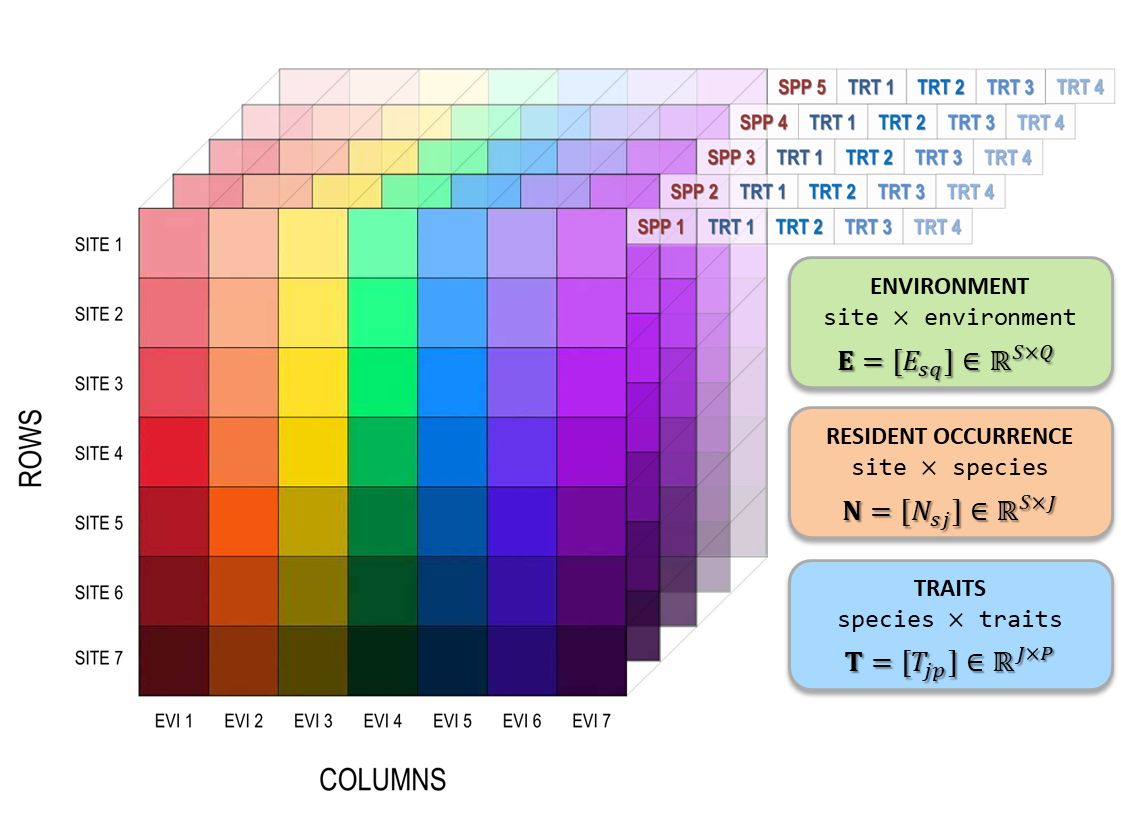
Figure 1: Data-cube schematic showing the three core matrices that are integrated into a unified multidimensional structure: - Environment $\mathbf{E}\in\mathbb{R}^{S\times Q}$ where for each site $s$, columns EVI1 to EVI5 are environmental variables (e.g., climate, soils) attached to that site’s location $(x_s,y_s)$ - Resident occurrence $\mathbf{N}\in\mathbb{R}^{S\times J}$ where for the same sites, columns SPP1 to SPP5 are species $j$ with abundance or occurrence recorded at site $s$ - Traits $\mathbf{T}\in\mathbb{R}^{J\times P}$ where for each species $j$, columns TRT1 to TRT4 are trait values (e.g., size, colour, life stage). $\mathbf{T}$ links to $\mathbf{N}$ via the shared species ID. - Stacking $\mathbf{E}$, $\mathbf{N}$, and $\mathbf{T}$ forms a consistent data cube that underpins trait-environment modeling and downstream invasion analyses.

Shared Trait-Environment Space

Integrating traits, environment, community composition and abundance (or presence-absence) into a unified framework, the multidimensional trait-environment space provides a geometric representation of these interactions, allowing invasion fitness to be visualised in spatial terms. In this way, each species occupies a region defined by its traits and ecological tolerances. In this space, each axis corresponds to a trait or environmental variable, and species are represented as points (or point clouds) defined by their values. In the shared trait space, ecological interactions and establishment potential can thus be understood through geometric measures:

The community forms a species cloud in trait space, whose shape reflects the diversity of resident strategies.
The convex hull of this cloud approximates the realised niche space.
Invasion fitness depends on an invader’s distance to the cloud centroid (trait centrality) and position relative to the hull.
Geometric measures (distances, overlaps, boundaries) map onto ecological processes: alignment with environment (abiotic suitability), niche crowding, and competitive displacement.

Within this framework, invasion fitness can be estimated using the geometry of trait space. That is, invaders positioned on the periphery or in under-occupied regions are more likely to establish, whereas those embedded within dense resident clusters experience stronger competition and lower fitness. Typically, fitness can be decomposed into three components (Figure 2):

Abiotic suitability - captures the alignment between the invader’s traits and the local environment.
Niche crowding - reflects the overlap with resident trait space, weighted by resident composition.
Resident competition (site saturation) - represents the competitive pressure from residents that already perform well at the site.

Invasion Fitness

Invasion fitness $(\lambda_{is})$ is a central concept in adaptive dynamics and eco-evolutionary theory, providing a predictor of coexistence, competitive exclusion, and adaptive evolutionary outcomes. It predicts whether species $i$ can take hold at site $s$ i.e. positive values suggest establishment, negative values suggest failure. More specifically, $\lambda_{is}$ is defined as the per capita growth rate of a rare species introduced into a resident community at ecological equilibrium. It combines the effects of abiotic suitability, niche crowding, and resident competition, to determine whether an invader $i$ with traits $\mathbf{t_i} \in \mathbb{R}^p$ can establish and persist at site $s$ with environmental conditions $\mathbf{e_s} \in \mathbb{R}^q$ and resident community composition $\mathbf{n_s} \in \mathbb{R}^j$. Mathematically, invasion fitness is expressed as:

Invasion fitness formula

where $r^{(z)}_{is}$ is the invader’s environmental fit at the site (standardised so values are comparable across sites and species). ➜ The coefficient $\Gamma_{is}$ tells how strongly that fit translates into potential growth.
The term $C^{(z)}_{is}$ measures niche crowding i.e. how much look-alike residents already occupy the same niche. ➜ $\alpha_{is}$ is how severely that overlap reduces the invader’s success.
The term $S^{(z)}_{is}$ reflects site saturation i.e. how “full” or dominance-skewed the community is. ➜ $\beta_i$ is the invader’s sensitivity to that general resident pressure.
$\kappa$ is a small calibration offset that sets the baseline (typically centering residents near zero) without changing relative rankings.|

💡 In short, $\lambda_{is}$ balances how suitable the site is against how hard it is to elbow in. When environmental benefits outweigh crowding and saturation penalties, $\lambda_{is}>0$ and establishment is more likely; when penalties dominate, $\lambda_{is}<0$.

Invasiveness and Invasibility

The invasion fitness output can be aggregated to site and species level summaries of invasiveness $V_i$ & $T_{ik}$ and invasibility $V_s$ to provide interpretable metrics for mapping and prioritisation;

Species Invasiveness is the proportion of sites ($S$) where species $i$ can establish i.e. it identifies trait combinations that enable broad establishment:

\[ V_i \;=\; \frac{1}{|S|} \sum_{s} \mathbb{I}\{\lambda_{is} > 0\} \]
Trait Invasiveness is how much a single trait explains variation in species invasiveness $V_i$ across species, yielding one scalar per trait e.g. for trait $T_k$ (the $k$-th trait):

\[ \mathrm{TI}_k \;=\; \frac{\mathrm{Var}\!\left(\mathbb{E}[\,V_i \mid T_{ik}\,]\right)}{\mathrm{Var}(V_i)} \] where invasiveness is the fraction of variance in $V_i$ explained by trait $T_k$ alone (no other covariates).
Site Invasibility is the proportion of invaders ($I$) that establish at site $s$ i.e. it identifies invasion “hotspots” or resistant communities.

\[ V_s \;=\; \frac{1}{|I|} \sum_{i} \mathbb{I}\{\lambda_{is} > 0\} \]

💡The decomposition of invasion fitness into abiotic suitability, niche crowding, and biotic resistance or resident competition, reinforces that successful invasion depends both on the compatibility of the invader (incl. its associated traits) with its abiotic environment and on the competitive structure of the biotic community. Thus, if invasion fitness is positive, the invader is expected to increase in abundance; if negative, it will fail to establish. In other words, $\lambda_{is} > 0$ implies positive invasion fitness, suggesting establishment of invader $i$ is possible at site $s$. Therefore a probabilistic measure of establishment can also be derived as:

\[ P(F>0) \;=\; \Phi\!\left(\frac{\mu_{is}}{\sigma}\right) \]

where $\mu_{is}$ is the predicted mean invasion fitness and $\sigma$ is the predictive residual standard deviation.

Overview of `invasimapr` workflow

The invasimapr workflow links raw ecological inputs (Figure 1) to decision-ready outputs, progressing from resident community data, traits $T$, abundances $N$ across sites $S$ with environments $E$, to site-level maps and species rankings (Figure 2). Each stage corresponds to wrapper functions implemented in specific scripts, so users can trace every conceptual step to its code. Intermediate objects are returned throughout for auditability and reuse.

Setup Install and load invasimapr from GitHub to make the full workflow available, alongside the core libraries used for spatial handling, biodiversity modelling, and visualisation. If you do not already have species-occurrence and/or environmental site data, install dissmapr (GitHub) for modular acquisition and preparation of biodiversity data. The utility wrapper utils_internal creates a pipeline container with new_invasimapr_fit(), prints a compact summary via print.invasimapr_fit(), and standardises predictors with .standardise_df(); together these utilities harmonise IDs and scales before modelling begins.
Data access and preparation You may read local data with utils::read.csv or use dissmapr to pull raw observations from GBIF, harmonise them onto spatial grids, and extract environmental predictors. get_trait_data() retrieves and aligns species traits (e.g. from Wikipedia-derived tables) so community, environment, and invader information integrate cleanly downstream. The wrapper prepare_inputs calls assemble_matrices() to build the core inputs, namely site coordinates, site × environment tables, site × resident matrices, and trait tables, while invader profiles are either imported or simulated with simulate_invaders() by resampling resident trait distributions.
Trait space and resident crowding The wrapper prepare_trait_space standardises model inputs and characterises the joint trait space, writing outputs to fit$traits and fit$crowding. standardise_model_inputs() z-scores environments and resident traits, rescales invader traits using resident means/SDs (preventing leakage), and aligns factor levels; outputs include env_df_z, traits_res_glmm, and traits_inv_glmm with scaling metadata. compute_trait_space() constructs a shared resident-invader trait map, compute_centrality_hull() computes centrality and convex-hull membership, and compute_resident_crowding() derives crowding indices $C_{js}$ from community composition and trait similarity (Gower to Gaussian kernel) with robust z-standardisation.
Resident modelling The model_residents wrapper fits resident responses to traits and environments. build_model_formula() defines a GLMM-ready formula; prep_resident_glmm() builds the site × resident long table and fits a residents-only GLMM to obtain link-scale suitability $r_{js}$ and expected abundances $\mu_{js}$. standardise_by_site() row-standardises site×species matrices, and compute_site_saturation() yields site-level saturation $S_s$ and its z-standardised form $S^{(z)}_s$.
Sensitivity estimation The learn_sensitivities wrapper estimates resident-only slopes and trait sensitivities. fit_auxiliary_residents_glmm() fits trait × predictor interactions with optional site random slopes; derive_sensitivities() extracts invader-level $\alpha_i$ (crowding), $\beta_i$ (saturation), $\theta_i$ (abiotic slope), and a fallback $\gamma_i$; and site_varying_alpha_beta_gamma() combines fixed effects with site deviations to produce $\alpha_{is}$ and $\Gamma_{is}$, while propagating $\beta_i$.
Invader predictors Using predict_invaders, the function build_invader_predictors() generates invader-specific predictors on the resident-calibrated scale: $r^{(z)}_{is}$ for abiotic suitability, $C^{(z)}_{is}$ for trait-weighted crowding, and $S^{(z)}_{is}$ for site saturation (broadcast across invaders).
Invasion fitness and establishment probability The wrapper predict_establishment assembles fitness and translates it to probability. compute_invasion_fitness() forms \[ \lambda_{is} \;=\; \Gamma_{is}\, r^{(z)}_{is} \;-\; \alpha_{is}\, C^{(z)}_{is} \;-\; \beta_i\, S^{(z)}_{is} \;+\; \kappa, \] allowing global or site-varying slopes, signed vs unsigned saturation effects, and calibration via $\kappa$ so resident mean $\lambda$ is zero. compute_establishment_probability() then maps $\lambda_{is}$ to $p_{is}$ using probit, logit, or hard thresholds, returning matrices aligned with $\lambda_{is}$.
Summarisation and interpretation Finally, summarise_results calls summarise_invasiveness_invasibility() to collapse site × invader surfaces into species invasiveness (mean breadth of establishment across sites), site invasibility (mean probability or fraction of invaders establishing), and trait-level associations (continuous slopes or ANOVA $R^2$ for categorical traits). Outputs include tidy species- and site-level tables, trait-effect summaries, and a suite of plots (e.g. maps, rankings, heatmaps, trait-effect diagrams), providing management-ready summaries and ecological insight.

invasimapr Workflow

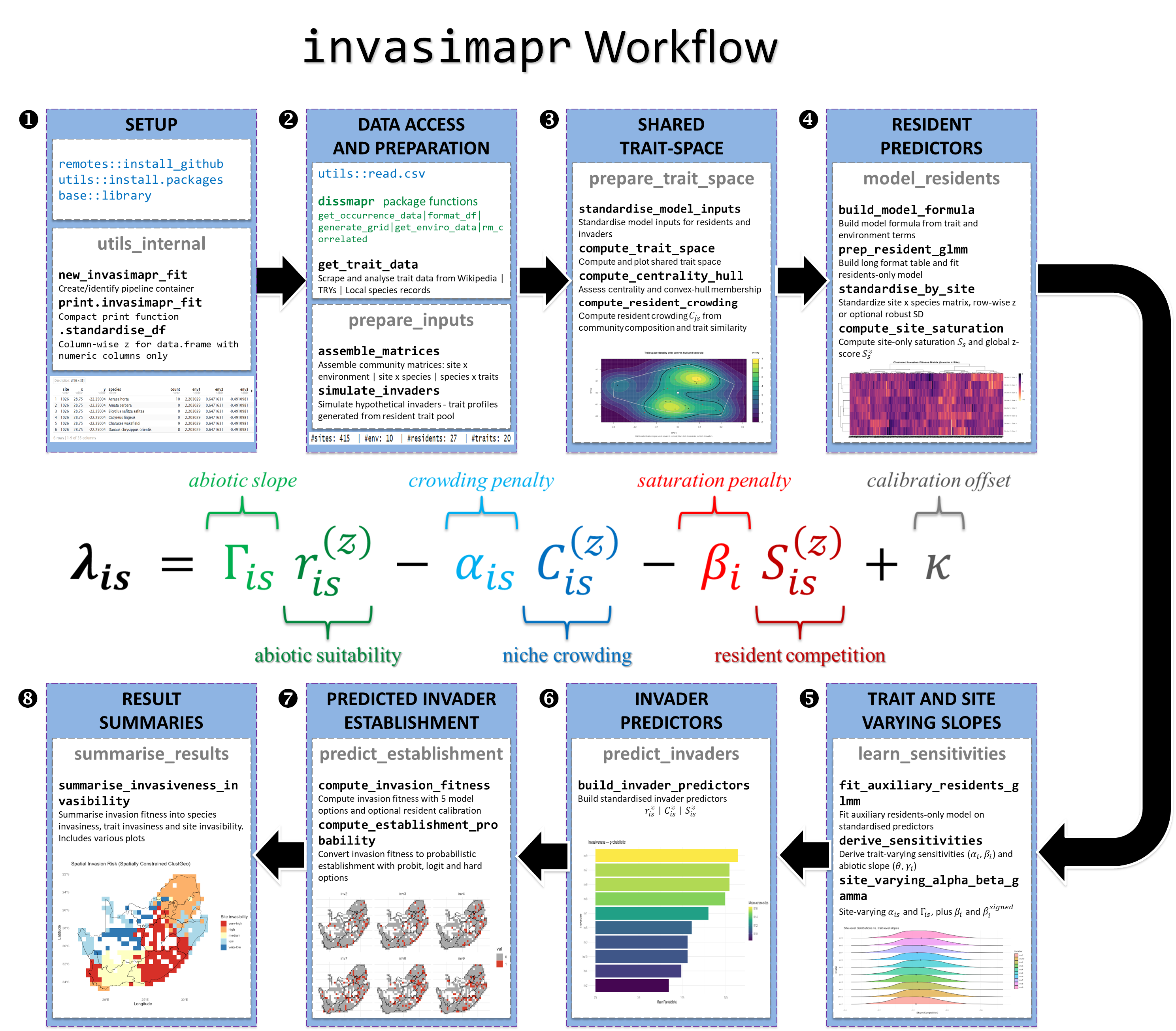
Figure 2: invasimapr workflow linking data access, preparation, trait-space modelling, resident predictors, and slope estimation to the invasion fitness equation - The invasion fitness formula decomposes into four components: abiotic suitability $\Gamma_{is} r^{(z)}_{is}$ (green), niche crowding penalty $-\alpha_{is} C^{(z)}_{is}$ (blue), resident saturation penalty $-\beta_i S^{(z)}_{is}$ (red), and a calibration offset $\kappa$ (grey). Each component is derived from specific workflow modules, converging on predicted invader establishment and summarised results, which provide actionable outputs to policy.

💡Across eight wrappers and eigthteen functions, invasimapr offers a logically ordered pipeline. Utility functions prepare and standardise inputs; resident and invader predictors are generated on common scales; invasion fitness and establishment probabilities are derived under flexible assumptions; and results are summarised into interpretable, map-ready outputs. Explicit mapping of each conceptual step to a wrapper function ensures reproducibility, transparency, and accessibility for both ecological research and applied biodiversity monitoring.

Discussion and conclusion

We presented a reproducible workflow, implemented in invasimapr, that links traits, environment, and community composition to invader establishment potential. The pipeline proceeds from aligned inputs (Section 2), to shared trait geometry and crowding (Section 3), to resident-only predictors (Section 4), trait- and site-varying sensitivities (Section 5), invader predictors (Section 6), invasion fitness and probabilities (Section 7), and decision-ready summaries (Section 8), with optional clustering and spatial risk scenarios (Sections 9-10).

Key insights.

A shared trait space (PCoA on Gower) provides a transparent lens on overlap vs. novelty; convex-hull and centrality diagnostics make this geometry interpretable.
Niche crowding $C$ (composition × similarity) captures biotic resistance, while abiotic suitability $r$ and site saturation $S$ supply complementary axes of opportunity and constraint.
Learning sensitivities ($\alpha, \beta, \Gamma/\gamma$) connects trait position (and optional site heterogeneity) to how strongly these axes matter, enabling multiple fitness specifications (A-E) without changing predictors.
Standardising invaders on resident moments prevents information leakage and ensures scales are comparable across species and sites.
Clustering compresses the prediction surface into invader types and site categories, which map naturally to surveillance and management priorities.

Assumptions and limitations: The approach assumes (i) trait coverage sufficient to represent functional niches; (ii) stationarity of trait-environment relationships across the spatial domain; (iii) crowding kernels that reasonably approximate similarity in competitive effects. Sensitivity to ordination choices, kernel bandwidth $\sigma_\alpha$, GLMM specification (e.g., Tweedie vs. alternatives), and the treatment of S should be checked. Where training data are sparse, drop overly rich $E\times T$ interactions or use penalised variants.

Validation and robustness: We recommend k-fold cross-validation by site blocks, posterior predictive checks for GLMMs, and ablation tests: (a) remove $C$ to quantify biotic resistance; (b) remove $S$ to isolate trait-specific crowding; (c) randomise trait labels to benchmark signal vs. noise. Compare fitness options (A-E) and report stability of ranks and maps.

Use in practice: For surveillance, target sites in high-risk categories and emphasise broad-spectrum invader types. For management, combine hotspots of high $r^{(z)}$ with low $C^{(z)}$ to identify windows of vulnerability, and track changes through time as communities or environments shift. The tidy outputs (tables + plots) are designed to support open reporting and iterative updates.

Future extensions: Incorporate temporal dynamics (seasonality, multi-year changes), explicit propagule pressure, alternative similarity kernels, and causal structure (e.g., SEM) to partition direct vs. mediated effects. Where data allow, integrate detection models for observation bias.

Conclusion: invasimapr operationalises a trait-centred, community-aware view of invasion risk. By keeping geometry, predictors, and coefficients transparent and aligned, the workflow bridges ecological interpretation and practical decision-making, delivering reproducible maps, ranks, and risk profiles that can evolve with new data.

:bulb: Final takeaway: Keep inputs aligned, scale invaders on resident moments, prefer fixed-effects predictions for comparability, and use clustering sparingly but purposefully to turn rich fitness surfaces into actionable categories.

References

Hui, C. (2016) Defining invasiveness and invasibility in ecological networks: invasion fitness = per-capita growth rate at trivial propagule size. (pure.iiasa.ac.at, SciSpace)
Hui, C. & Richardson, D. (2023) Disentangling the relationships among abundance, occupancy and invasiveness: invasiveness measured by expected initial per-capita population growth rate (“invasion growth rate”). (Nature)
Hui, C. (2021) Trait positions for elevated invasiveness in adaptive ecological networks: extends invasion-fitness concept in an adaptive-dynamics/network setting. (SpringerLink, pure.ed.ac.uk)
Landi, P., Dercole, F., Rinaldi, S. (2013) Branching scenarios… IIASA IR-13-044: invasion fitness $\lambda_i$ = initial exponential rate of increase of the mutant; appears in the canonical equation. (pure.iiasa.ac.at)
Landi, P. et al. (2018) Variability in life-history switch points…: invasion fitness framed as expected offspring number per generation (discrete-time analogue). (PMC)

Appendices

Expanded formula and links to model components

We summarize how each component of the invasion fitness function is computed, linking back to the ecological quantities and trait dependence.

\[ \boxed{\; \lambda_{is} \;=\; \underbrace{\gamma_i}_{\text{slope on suitability}} \;\;\underbrace{r^{(z)}_{is}}_{\text{trait-conditioned suitability}} \;-\; \underbrace{\alpha_i}_{\text{slope on crowding}} \;\;\underbrace{C^{(z)}_{is}}_{\text{trait-space crowding}} \;-\; \underbrace{\beta_i}_{\text{slope on filtering}} \;\;\underbrace{S^{(z)}_{is}}_{\text{performance-weighted filtering}} \;} \]

Here $\gamma_i, \alpha_i, \beta_i$ are trait-dependent slopes, evaluated at invader traits $t_i$, and $r^{(z)}_{is}, C^{(z)}_{is}, S^{(z)}_{is}$ are site-invader predictors derived from resident data but conditioned on invader traits $t_i$.

Trait-conditioned environmental suitability $r^{(z)}_{is}$

Resident $E \times T$ model: Fit on residents $j$,

\[ r_{js} = \text{FE}_{E \times T}(\text{env}_s, t_j), \]

where $\text{FE}_{E \times T}$ is the fixed-effect surface of environment × trait predictors.
Invader projection: Evaluate at invader traits $t_i$:

\[ r_{is} = \text{FE}_{E \times T}(\text{env}_s, t_i). \]
Resident-anchored z-score:

\[ r^{(z)}_{is} = \frac{r_{is} - \mu_r}{\sigma_r}, \]

where $\mu_r, \sigma_r$ are mean and SD across resident species at site $s$.

Trait-space crowding $C^{(z)}_{is}$

Kernel overlap in trait space:

\[ K_{ir} = \exp\!\left\{-\frac{d^2(t_i,t_j)}{2\tau^2}\right\}, \]

where $d(t_i,t_j)$ is trait distance, $\tau$ a bandwidth.
Site composition weights: $W_{\text{site}}(s,j)$ (Hellinger-scaled abundances).
Crowding index:

\[ C_{is} = \sum_j K_{ir}\, W_{\text{site}}(s,j). \]
Resident-anchored z-score:

\[ C^{(z)}_{is} = \frac{C_{is} - \mu_C}{\sigma_C}. \]

Performance-weighted resident filtering $S^{(z)}_{is}$

Neighbor performance signal: Residents’ site-specific suitability $r_{js}$.
Implemented sum (code):

\[ S_{is} = \sum_j K_{ir}\; r_{is}\; r_{js}\; W_{\text{site}}(s,j). \]

(This form includes both invader and resident suitability; a pure neighbor filter would omit $r_{is}$).
Resident-anchored z-score:

\[ S^{(z)}_{is} = \frac{S_{is} - \mu_S}{\sigma_S}. \]

Trait-dependent slopes $\gamma_i, \alpha_i, \beta_i$

Auxiliary regression on residents:

\[ \log(1+\text{abund}_{js}) \sim (r^{(z)} + C^{(z)} + S^{(z)}) \times (\text{tr1} + \text{tr2}) \;+\; (1|\text{species}) + (1|\text{site}). \]
Linear slope surfaces in trait space:

\[ \gamma(t) = b_{r,0} + b_{r,1}\,t_1 + b_{r,2}\,t_2, \quad \alpha(t) = b_{C,0} + b_{C,1}\,t_1 + b_{C,2}\,t_2, \quad \beta(t) = b_{S,0} + b_{S,1}\,t_1 + b_{S,2}\,t_2. \]
Invader-specific slopes: $\gamma_i = \gamma(t_i), \; \alpha_i = \alpha(t_i), \; \beta_i = \beta(t_i).$

Predictive distribution

Mean invasion fitness: $\mu_{is} = \lambda_{is}.$
Delta-method predictive variance: $\sigma^2_{\text{pred},is}$ from fixed-effect covariance + residual.
Probability of establishment:

\[ P(F>0) \;\approx\; \Phi\!\left(\frac{\mu_{is}}{\sigma_{\text{pred},is}}\right). \]

Glossary (objects and equation components)

Symbol / Term	R Object(s)	Definition	Relevance
$r_{js}$	`r_js`	Resident FE-only predictor (link scale) from E×T GLMM	Baseline suitability per resident & site
$r_{is}$	`r_is`	Invader FE-only predictor (projected)	Invader suitability before scaling; becomes $r^{(\tilde{t})}_{is}$ after z-scoring
Resident scaling moments	`r_mu`,`r_sd`; `C_mu`,`C_sd`; `S_mu`,`S_sd`	Means/SDs computed on residents only	Used to standardise invader predictors, preventing leakage
$r^{(\tilde{t})}_{is}$	`r_is_z`	standardised invader suitability	Feeds $\gamma_i r^{(\tilde{t})}_{is}$
$C_{is}$	`C_is`	Trait-kernel exposure $W_{\text{site}} K_{ri}^\top$	Crowding/overlap pressure
$C^{(\tilde{t})}_{is}$	`C_is_z`	standardised crowding	Feeds $\alpha_i C^{(\tilde{t})}_{is}$
$S_{js}$	`S_js`	Resident convolution $K_{\text{res}}\cdot (r_{js}\odot W_{\text{site}})$	Neighbor success signal by resident & site
$S_{is}$	`S_is`	Invader-resident interaction sum $\sum_j K_{ij}\,r_{is}\,r_{js}\,W_{sj}$	Site × invader filtering pressure
$S^{(\tilde{t})}_{is}$	`S_is_z`	standardised filtering	Feeds $\beta_i S^{(\tilde{t})}_{is}$
$\gamma_i,\alpha_i,\beta_i$	`gamma_i`,`alpha_i`,`beta_i`	Trait-varying slopes (linear in `tr1/2`)	Transfer strength of each standardised component to fitness
$\mu_{is}$	`MU` / `pe$mu`	Mean fitness on standardised scale	Center for Normal approximation
$\sigma$	`pe$sigma`	Predictive SD from auxiliary model	Scale for $P(F>0)=\Phi(\mu/\sigma)$
$P(F>0)$	`pe$p_establish`	Probabilistic establishment matrix (site × invader)	Used for mapping, ranking, calibration
$D_s$	`D_s`	Site density/productivity proxy (row sums)	Confounder separated from `C_is` upstream
$Q_s$	`Q_s`	Abiotic propensity (mean `r_js` per site)	Confounder separated from `C_is` upstream; optional residualization
$\tau$	`tau_hat`, `tau_grid`	Kernel bandwidth estimated from resident distance-overlap	Sets the scale of trait-based crowding and filtering
LOSO outputs	`loso_fast`, `loso_cal`	Per-site probabilities and calibration table	Backtesting transferability and reliability

Introduction

`invasimapr`

A novel framework to visualise trait dispersion and assess species invasiveness and site invasibility

Introduction

Network Invasibility Cube

Shared Trait-Environment Space

Invasion Fitness

Invasiveness and Invasibility

Overview of `invasimapr` workflow

Discussion and conclusion

References

Appendices

Expanded formula and links to model components

Trait-conditioned environmental suitability \(r^{(z)}_{is}\)

Trait-space crowding \(C^{(z)}_{is}\)

Performance-weighted resident filtering \(S^{(z)}_{is}\)

Trait-dependent slopes \(\gamma_i, \alpha_i, \beta_i\)

Predictive distribution

Glossary (objects and equation components)

Symbol / Term	R Object(s)	Definition	Relevance
\(r_{js}\)	`r_js`	Resident FE-only predictor (link scale) from E×T GLMM	Baseline suitability per resident & site
\(r_{is}\)	`r_is`	Invader FE-only predictor (projected)	Invader suitability before scaling; becomes \(r^{(\tilde{t})}_{is}\) after z-scoring
Resident scaling moments	`r_mu`,`r_sd`; `C_mu`,`C_sd`; `S_mu`,`S_sd`	Means/SDs computed on residents only	Used to standardise invader predictors, preventing leakage
\(r^{(\tilde{t})}_{is}\)	`r_is_z`	standardised invader suitability	Feeds \(\gamma_i r^{(\tilde{t})}_{is}\)
\(C_{is}\)	`C_is`	Trait-kernel exposure \(W_{\text{site}} K_{ri}^\top\)	Crowding/overlap pressure
\(C^{(\tilde{t})}_{is}\)	`C_is_z`	standardised crowding	Feeds \(\alpha_i C^{(\tilde{t})}_{is}\)
\(S_{js}\)	`S_js`	Resident convolution \(K_{\text{res}}\cdot (r_{js}\odot W_{\text{site}})\)	Neighbor success signal by resident & site
\(S_{is}\)	`S_is`	Invader-resident interaction sum \(\sum_j K_{ij}\,r_{is}\,r_{js}\,W_{sj}\)	Site × invader filtering pressure
\(S^{(\tilde{t})}_{is}\)	`S_is_z`	standardised filtering	Feeds \(\beta_i S^{(\tilde{t})}_{is}\)
\(\gamma_i,\alpha_i,\beta_i\)	`gamma_i`,`alpha_i`,`beta_i`	Trait-varying slopes (linear in `tr1/2`)	Transfer strength of each standardised component to fitness
\(\mu_{is}\)	`MU` / `pe$mu`	Mean fitness on standardised scale	Center for Normal approximation
\(\sigma\)	`pe$sigma`	Predictive SD from auxiliary model	Scale for \(P(F>0)=\Phi(\mu/\sigma)\)
\(P(F>0)\)	`pe$p_establish`	Probabilistic establishment matrix (site × invader)	Used for mapping, ranking, calibration
\(D_s\)	`D_s`	Site density/productivity proxy (row sums)	Confounder separated from `C_is` upstream
\(Q_s\)	`Q_s`	Abiotic propensity (mean `r_js` per site)	Confounder separated from `C_is` upstream; optional residualization
\(\tau\)	`tau_hat`, `tau_grid`	Kernel bandwidth estimated from resident distance-overlap	Sets the scale of trait-based crowding and filtering
LOSO outputs	`loso_fast`, `loso_cal`	Per-site probabilities and calibration table	Backtesting transferability and reliability

Introduction

invasimapr

A novel framework to visualise trait dispersion and assess species invasiveness and site invasibility

Introduction

Network Invasibility Cube

Shared Trait-Environment Space

Invasion Fitness

Invasiveness and Invasibility

Overview of invasimapr workflow

Discussion and conclusion

References

Appendices

Expanded formula and links to model components

Trait-conditioned environmental suitability \(r^{(z)}_{is}\)

Trait-space crowding \(C^{(z)}_{is}\)

Performance-weighted resident filtering \(S^{(z)}_{is}\)

Trait-dependent slopes \(\gamma_i, \alpha_i, \beta_i\)

Predictive distribution

Glossary (objects and equation components)

`invasimapr`

Overview of `invasimapr` workflow