Get started with dissmapr

dissmapr provides a reproducible, end-to-end workflow for computing and mapping compositional dissimilarity and biodiversity turnover across large spatial scales. This short guide runs a complete, self-contained workflow on the example GBIF butterfly dataset for South Africa that ships with the package, taking you from raw occurrence records to a gridded species-richness map.

For the full, step-by-step tutorials (environmental linking, zeta diversity, MS-GDM, bioregional mapping and change detection), see the Articles on the package website.

Installation

# install.packages("remotes")
remotes::install_github("b-cubed-eu/dissmapr")

A minimal, reproducible workflow

library(dissmapr)

# 1. Load the example occurrence dataset shipped with the package
load(system.file("extdata", "gbif_butterflies_csv.RData", package = "dissmapr"))

# 2. Import and harmonise the occurrence records
occ <- get_occurrence_data(
  data        = gbif_butterflies_csv,
  source_type = "data_frame"
)

# 3. Reshape into long (site_obs) and wide (site_spp) tables
fmt <- format_df(
  data        = occ,
  species_col = "verbatimScientificName",
  value_col   = "pa",
  format      = "long"
)
site_spp <- fmt$site_spp

# 4. Summarise records onto a 0.5-degree grid
grid <- generate_grid(
  data      = site_spp,
  x_col     = "x",
  y_col     = "y",
  grid_size = 0.5,
  sum_cols  = 4:ncol(site_spp),
  crs_epsg  = 4326
)

# 5. Map gridded species richness
terra::plot(grid$grid_r[["spp_rich"]],
            main = "Butterfly species richness (0.5° grid)")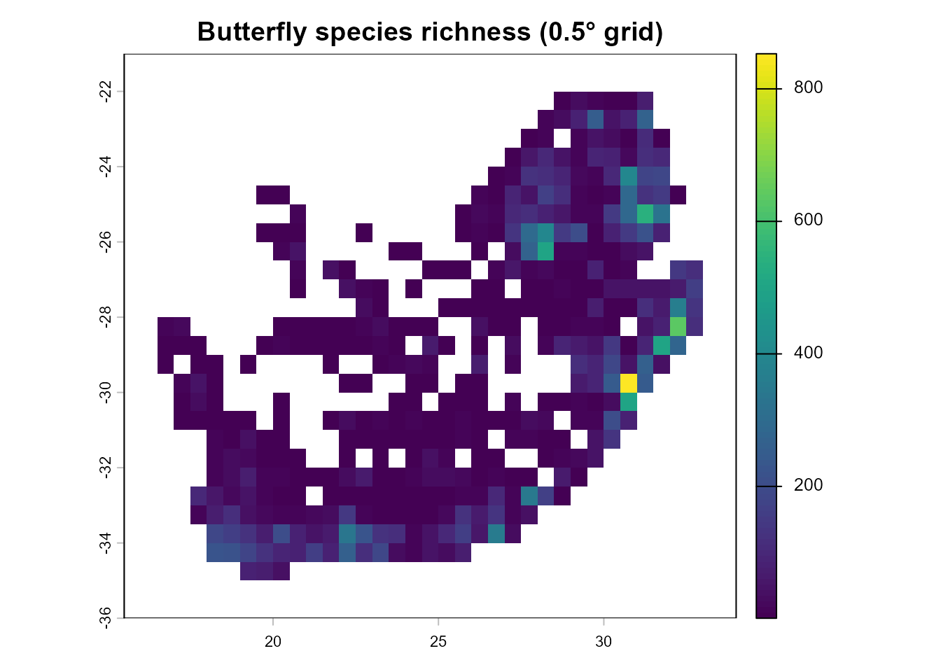

Each function can be used on its own or chained into an end-to-end pipeline. From here, the Articles walk through the rest of the workflow in detail.