
dissmapr
Delineating Bioregions from Predicted Community Composition
This vignette shows how predicted compositional patterns can be translated into biodiversity regions. By grouping areas with similar predicted communities, the workflow supports spatial interpretation of turnover patterns and highlights broad biogeographic structure.
To keep the example reproducible and quick to run, we use a small set
of example objects bundled with dissmapr. The setup chunk
below loads the required packages, reads the bundled data snapshot, and
unpacks the rasters, boundary data, and species information needed for
the bioregionalisation examples.
# Load the packages used in this vignette.
library(dissmapr)
library(terra)
library(RColorBrewer)

# Load the bundled example data snapshot.
inputs = readRDS(system.file("extdata", "dissmapr_vignettes.rds", package = "dissmapr"))

# Unpack the example objects used below.
predictors_df = inputs$predictors_df       # Environmental predictor values
all_preds = inputs$all_preds               # Model prediction outputs
rsa = inputs$rsa                           # South Africa boundary
grid_spp = inputs$grid_spp                 # Grid-level species data
sp_cols = inputs$sp_cols                   # Species column names

# Recreate the masked raster grid and load the future nearest-neighbour raster.
grid_masked = terra::mask(
  terra::setValues(
    terra::rast(system.file("extdata", "grid_r.tif", package = "dissmapr"))[[1]],
    1
  ),
  terra::vect(rsa)
)

future_nn = terra::rast(
  system.file("extdata", "future_nn.tif", package = "dissmapr")
)
1. Run clustering analyses using map_bioreg() to map
bioregions
In this step we translate our site‐level ζ₂ predictions into spatial
bioregions. Calling map_bioreg() on the predictors_df does
the following:
- z-scales the predicted turnover, longitude and latitude;
- fits four clustering algorithms (k-means, PAM, hierarchical and GMM);
- k-means partitions points around centroids and is fast for large data sets.
- PAM (Partitioning Around Medoids) is a medoid-based analogue of k-means that is more robust to outliers.
- Hierarchical agglomerative clustering builds a dendrogram and then “cuts” it at the chosen k, capturing nested structure in the data.
- GMM (Gaussian Mixture Model) treats clusters as multivariate normal distributions and assigns each point by maximum likelihood.
- realigns each method’s labels to the k-means solution for consistency;
- builds both nearest-neighbour and thin-plate-spline interpolated surfaces;
- returns the raw cluster assignments and gridded rasters, and—because
show_plot=TRUE—draws a 2×2 panel of maps.
The result is a set of complementary bioregion maps and rasters you can use to compare how different algorithms partition the landscape based on compositional turnover and geography.
# Add this to {, fig.width=11.25, fig.height=9, warning=FALSE, message=FALSE}
# Run `map_bioreg` function to generate and plot clusters
bioreg_current = dissmapr::map_bioreg(
  data = predictors_df,
  scale_cols = c("pred_zetaExp", "centroid_lon", "centroid_lat"),
  method = 'all', # Options: c("kmeans","pam","hclust","gmm","all"),
  k_override  = 8,
  interpolate = 'nn', # Options: c("none","nn","tps","all"),
  x_col ='centroid_lon',
  y_col ='centroid_lat',
  res = 0.5,
  crs = "EPSG:4326",
  plot = TRUE,
  bndy_fc = rsa)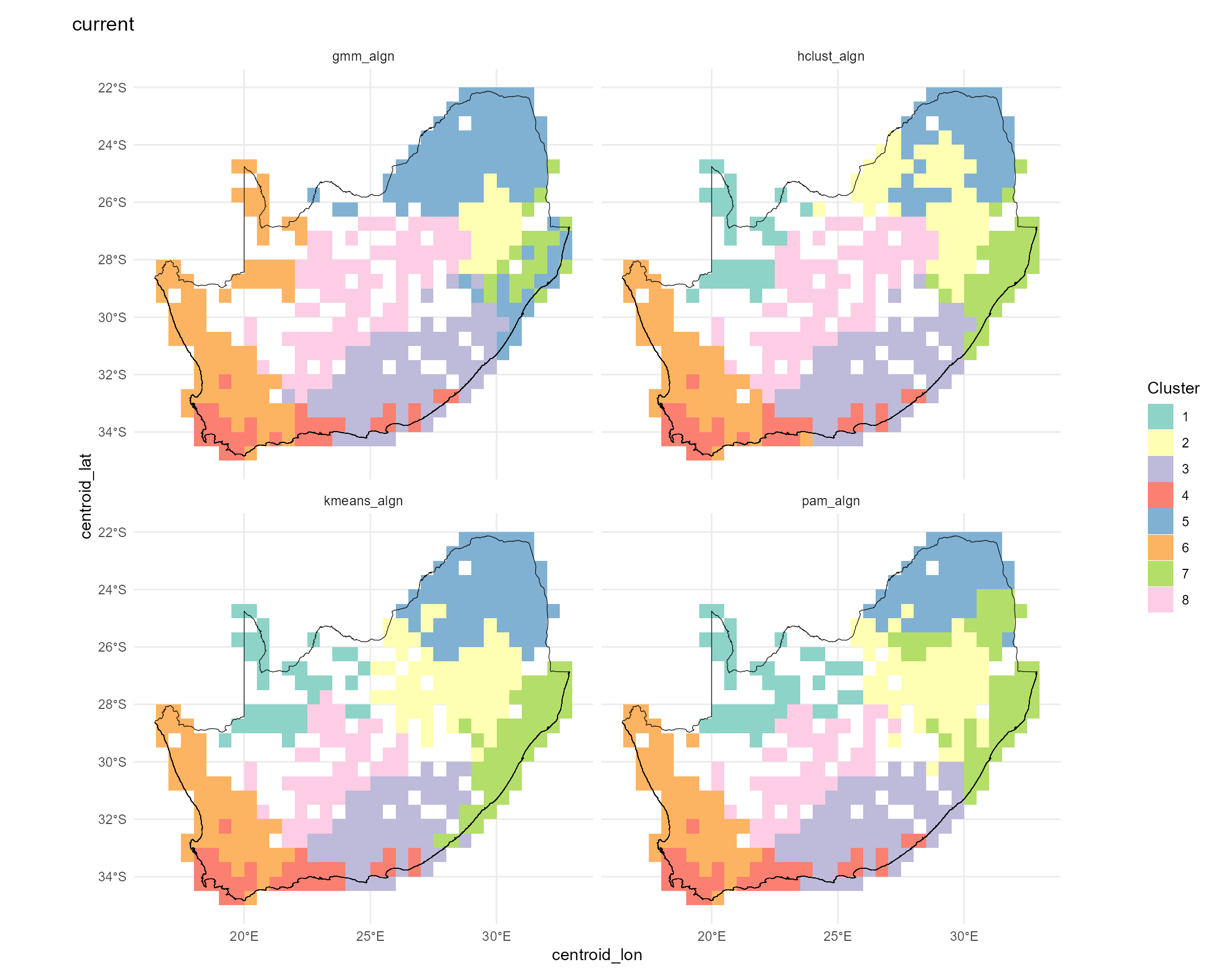
# Check results
str(bioreg_current, max.level=1)
#> List of 6
#>  $ none   :List of 1
#>  $ nn     :List of 1
#>  $ tps    : NULL
#>  $ table  :'data.frame': 415 obs. of  24 variables:
#>  $ plots  :List of 1
#>  $ methods: chr [1:4] "kmeans" "pam" "hclust" "gmm"
2. Map future bioregions using map_bioreg()
Below we expand our workflow to map the forecasted ζ₂ bioregions
under three extreme climate futures (2030, 2040, 2050) alongside the
current scenario. To see how the bioregional partitions shift, we split
all_preds by scenario and apply map_bioreg()
(k-means + hierarchical, both NN and TPS interpolation). We then extract
the hierarchical cluster layers, mask them to our study area, and plot
all four maps in a 2×2 layout:
# Split your combined predictions by scenario into a named list
by_scn = split(all_preds, all_preds$scenario)

# For each scenario, call map_bioreg() with all algorithms
bioreg_future = dissmapr::map_bioreg(
  data = by_scn,
  scale_cols = c("pred_zetaExp", "centroid_lon", "centroid_lat"),
  method = 'all', # Options: c("kmeans","pam","hclust","gmm","all"),
  k_override  = 8,
  interpolate = 'nn', # Options: c("none","nn","tps","all"),
  x_col ='centroid_lon',
  y_col ='centroid_lat',
  res = 0.5,
  crs = "EPSG:4326",
  plot = FALSE,
  bndy_fc = rsa)

# Check results
str(bioreg_future, max.level=1)
#> List of 6
#>  $ none   :List of 4
#>  $ nn     :List of 4
#>  $ tps    : NULL
#>  $ table  :'data.frame': 1660 obs. of  24 variables:
#>  $ plots  : NULL
#>  $ methods: chr [1:4] "kmeans" "pam" "hclust" "gmm"

# Plot the consensus bioregion clusters per scenario with a single, compact
# shared legend. Bioregions are categorical, so we keep a discrete key (Set3)
# rather than a continuous colour bar.
library(ggplot2)

clust_tbl = bioreg_future$table

# Order scenarios with "current" first, if present
scn_lev = unique(clust_tbl$scenario)
scn_lev = c(intersect("current", scn_lev), setdiff(scn_lev, "current"))
clust_tbl$scenario = factor(clust_tbl$scenario, levels = scn_lev)

ggplot() +
  geom_tile(data = clust_tbl,
            aes(x = centroid_lon, y = centroid_lat,
                fill = factor(cluster_mode))) +
  geom_sf(data = rsa, fill = NA, colour = "black", linewidth = 0.3) +
  facet_wrap(~ scenario) +
  scale_fill_brewer(palette = "Set3", name = "Bioregion", drop = FALSE) +
  theme_minimal(base_size = 9) +
  theme(legend.position = "bottom") +
  guides(fill = guide_legend(nrow = 1)) +
  labs(x = "Longitude", y = "Latitude")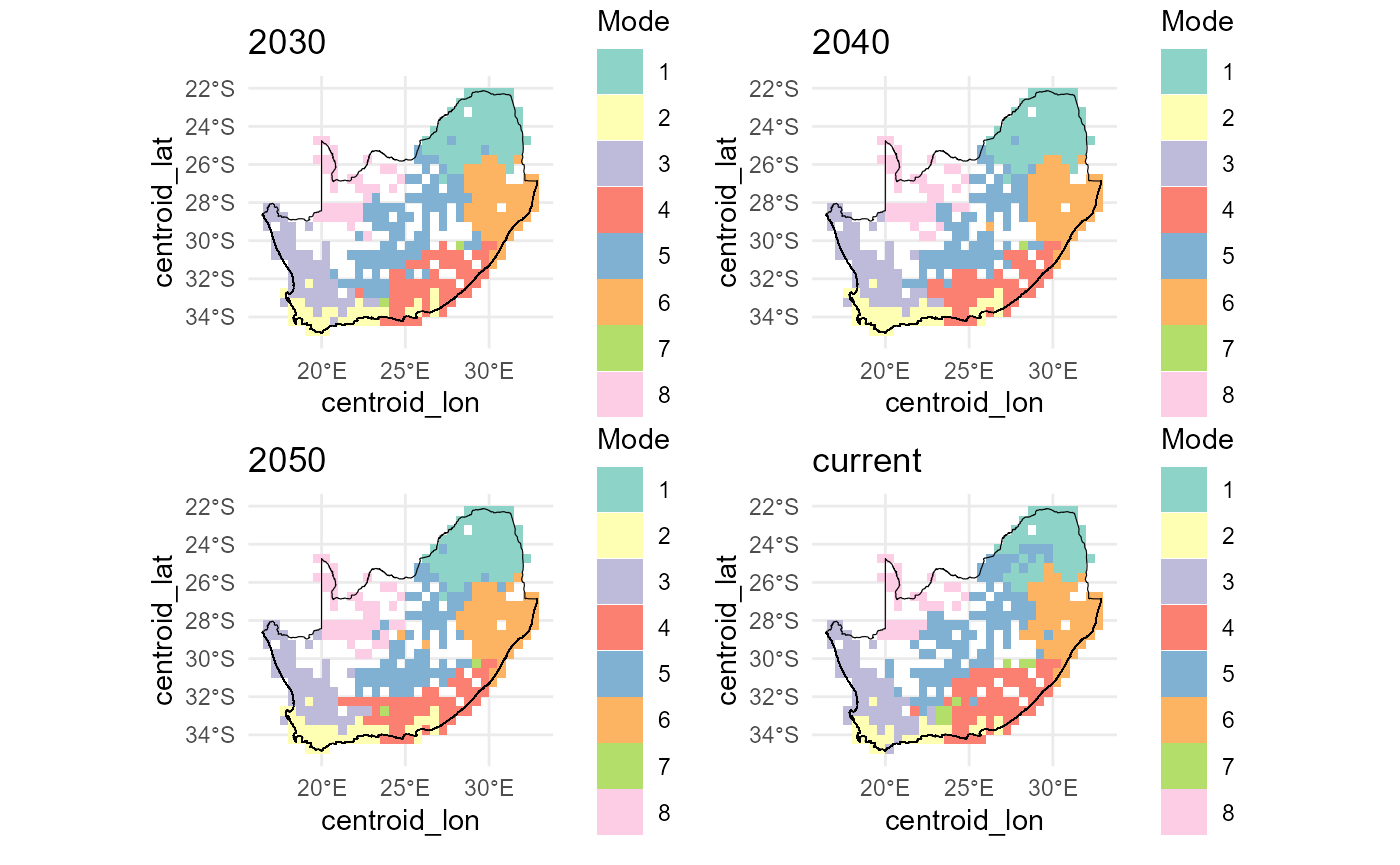
Below we visualise the nearest-neighbour interpolated future‐scenario
cluster outputs. First, we list the structure of the
bioreg_future result to confirm available components. We
then combine the k-means nearest-neighbour rasters for “current” and
each future year into a single SpatRaster stack
(future_nn), and resample, then mask it to the RSA boundary
(mask_future_nn). Finally, we lay out a 2×2 plot grid,
compute a discrete colour palette for each layer based on its unique
classes, and render each masked layer with its boundary overlay for a
quick inspection of bioregion changes across time.
# Check results
str(bioreg_future, max.level=1)
#> List of 6
#>  $ none   :List of 4
#>  $ nn     :List of 4
#>  $ tps    : NULL
#>  $ table  :'data.frame': 1660 obs. of  24 variables:
#>  $ plots  : NULL
#>  $ methods: chr [1:4] "kmeans" "pam" "hclust" "gmm"

# Create SpatRast
# future_nn = c(bioreg_future$nn$current$kmeans_current,
#              bioreg_future$nn$`2030`$kmeans_2030,
#              bioreg_future$nn$`2040`$kmeans_2040,
#              bioreg_future$nn$`2050`$kmeans_2050)
names(future_nn)
#> [1] "kmeans_current" "kmeans_2030"    "kmeans_2040"    "kmeans_2050"

# 4) Mask `result_bioregDiff` to the RSA boundary
mask_future_nn = terra::mask(resample(future_nn, grid_masked, method = "modal"), grid_masked)

# 5) Quick visual QC in a 2×2 layout
old_par = par(mfrow = c(2, 2), mar = c(1, 1, 1, 5))
titles = c("Current",
            "2030",
            "2040",
            "2050")

for (i in 1:4) {
  ## 1. how many distinct classes in this layer?
  cls  = sort(unique(values(mask_future_nn[[i]])))
  cls  = cls[!is.na(cls)]
  n    = length(cls)

  ## 2. build a discrete palette of n colours
  pal = if (n <= 12) {
           RColorBrewer::brewer.pal(n, "Set3")                      # native Set3
         } else {
           colorRampPalette(brewer.pal(12, "Set3"))(n) # extended Set3
         }

  ## 3. plot
  plot(mask_future_nn[[i]],
       col      = pal,
       type     = "classes",          # treats values as categories
       colNA    = NA,
       axes     = FALSE,
       legend   = TRUE,
       main     = titles[i],
       cex.main = 0.8)

  plot(terra::vect(rsa), add = TRUE, border = "black", lwd = .4)
}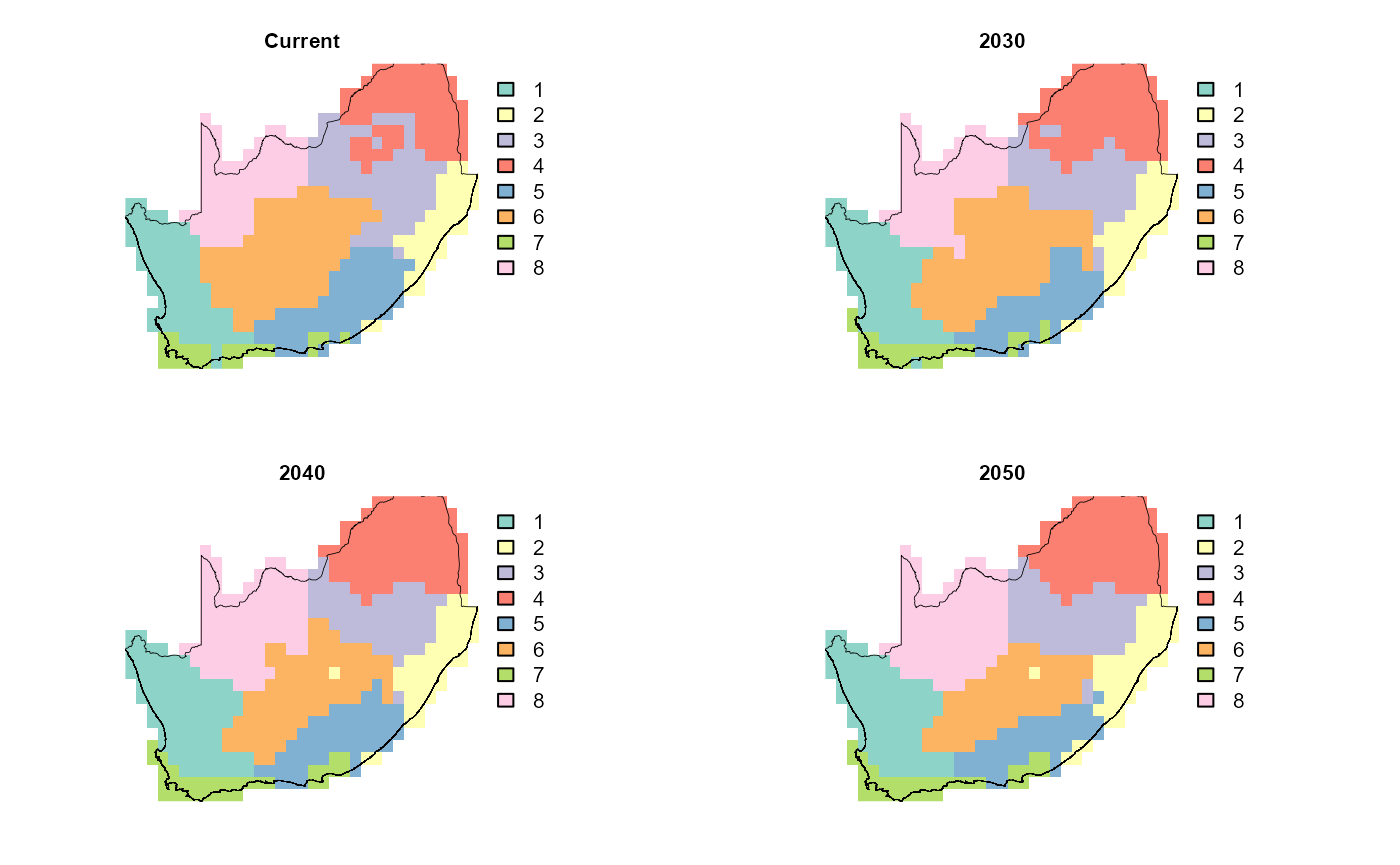
par(old_par)This end-to-end workflow shows how predicted turnover patterns and resulting bioregions might shift as climate warms and rainfall changes, highlighting potential future reorganization of biodiversity hotspots.
sessionInfo()
#> R version 4.5.2 (2025-10-31 ucrt)
#> Platform: x86_64-w64-mingw32/x64
#> Running under: Windows 11 x64 (build 26200)
#>
#> Matrix products: default
#>   LAPACK version 3.12.1
#>
#> locale:
#> [1] LC_COLLATE=English_South Africa.utf8  LC_CTYPE=English_South Africa.utf8
#> [3] LC_MONETARY=English_South Africa.utf8 LC_NUMERIC=C
#> [5] LC_TIME=English_South Africa.utf8
#>
#> time zone: Africa/Johannesburg
#> tzcode source: internal
#>
#> attached base packages:
#> [1] stats     graphics  grDevices datasets  utils     methods   base
#>
#> other attached packages:
#> [1] ggplot2_4.0.3      RColorBrewer_1.1-3 terra_1.9-34       dissmapr_0.2.0
#>
#> loaded via a namespace (and not attached):
#>   [1] DBI_1.3.0            pbapply_1.7-4        geodata_0.6-9
#>   [4] pROC_1.19.0.1        permute_0.9-10       rlang_1.2.0
#>   [7] magrittr_2.0.5       otel_0.2.0           e1071_1.7-17
#>  [10] compiler_4.5.2       mgcv_1.9-4           systemfonts_1.3.2
#>  [13] vctrs_0.7.3          maps_3.4.3           reshape2_1.4.5
#>  [16] stringr_1.6.0        pkgconfig_2.0.3      fastmap_1.2.0
#>  [19] rmarkdown_2.31       prodlim_2026.03.11   ragg_1.5.2
#>  [22] purrr_1.2.2          xfun_0.59            cachem_1.1.0
#>  [25] jsonlite_2.0.0       recipes_1.3.3        parallel_4.5.2
#>  [28] cluster_2.1.8.2      R6_2.6.1             bslib_0.11.0
#>  [31] stringi_1.8.7        parallelly_1.47.0    rpart_4.1.27
#>  [34] estimability_1.5.1   lubridate_1.9.5      jquerylib_0.1.4
#>  [37] Rcpp_1.1.1-1.1       iterators_1.0.14     knitr_1.51
#>  [40] future.apply_1.20.2  fields_17.3          zoo_1.8-15
#>  [43] Matrix_1.7-5         splines_4.5.2        nnet_7.3-20
#>  [46] timechange_0.4.0     tidyselect_1.2.1     rstudioapi_0.19.0
#>  [49] yaml_2.3.12          vegan_2.7-5          timeDate_4052.112
#>  [52] codetools_0.2-20     listenv_1.0.0        lattice_0.22-9
#>  [55] tibble_3.3.1         plyr_1.8.9           withr_3.0.3
#>  [58] S7_0.2.2             geosphere_1.6-8      evaluate_1.0.5
#>  [61] sf_1.1-1             future_1.70.0        desc_1.4.3
#>  [64] survival_3.8-6       units_1.0-1          proxy_0.4-29
#>  [67] mclust_6.1.2         pillar_1.11.1        KernSmooth_2.23-26
#>  [70] corrplot_0.95        renv_1.1.4           foreach_1.5.2
#>  [73] stats4_4.5.2         generics_0.1.4       zetadiv_1.3.0
#>  [76] scales_1.4.0         xtable_1.8-8         globals_0.19.1
#>  [79] class_7.3-23         glue_1.8.1           clValid_0.7
#>  [82] emmeans_2.0.3        tools_4.5.2          data.table_1.18.4
#>  [85] ModelMetrics_1.2.2.2 gower_1.0.2          mvtnorm_1.4-1
#>  [88] fs_2.1.0             dotCall64_1.2        grid_4.5.2
#>  [91] tidyr_1.3.2          ipred_0.9-15         nlme_3.1-169
#>  [94] patchwork_1.3.2      cli_3.6.6            rappdirs_0.3.4
#>  [97] textshaping_1.0.5    NbClust_3.0.1        spam_2.11-4
#> [100] viridisLite_0.4.3    scam_1.2-22          lava_1.9.1
#> [103] dplyr_1.2.1          gtable_0.3.6         sass_0.4.10
#> [106] digest_0.6.39        classInt_0.4-11      caret_7.0-1
#> [109] ggrepel_0.9.8        htmlwidgets_1.6.4    farver_2.1.2
#> [112] entropy_1.3.2        htmltools_0.5.9      pkgdown_2.2.0
#> [115] lifecycle_1.0.5      factoextra_2.0.0     hardhat_1.4.3
#> [118] httr_1.4.8           MASS_7.3-65