
dissmapr
Extracting Environmental Predictors for Biodiversity Modelling
This vignette shows how to attach environmental predictor data to the analysis grid. These predictors provide the environmental context needed for modelling spatial patterns in biodiversity, compositional turnover, and species richness.
To keep the example reproducible and quick to run, we use a small set
of example objects bundled with dissmapr. The setup chunk
below loads the required packages, reads the bundled data snapshot, and
unpacks the spatial, species, and raster objects needed for the
environmental-data workflow.
# Load the packages used in this vignette.
library(dissmapr)
library(ggplot2)
library(dplyr)

# Load the bundled example data snapshot.
# This keeps the vignette reproducible and avoids requiring external downloads.
inputs = readRDS(system.file("extdata", "dissmapr_vignettes.rds", package = "dissmapr"))

# Unpack the example objects used throughout this vignette:
# Unpack the bundled example data into named objects used below.
rsa = inputs$rsa                         # South Africa boundary
grid_sf = inputs$grid_sf                 # Analysis grid as an sf object
grid_spp = inputs$grid_spp               # Grid-level species data
effRich_r = terra::unwrap(inputs$effRich_r) # Effective richness raster
grid_spp_pa = inputs$grid_spp_pa         # Presence-absence species data
sp_cols = inputs$sp_cols                 # Species column names
grid_r = terra::rast(system.file("extdata", "grid_r.tif", package = "dissmapr")) # Raster template
1. Generate site by environment matrix using
get_enviro_data()
Spatial models are most informative when each sampling unit couples a
biological response (in this example, sampling effort
and species richness) with the same suite of
environmental predictors.get_enviro_data() attaches environmental predictors to each
grid cell via a six-stage routine:
o buffer the analysis lattice,
o retrieve or read the required rasters,
o crop them to the buffered extent,
o extract raster values at every grid-cell
centroid,
o interpolate any missing data gaps, and
o append the finished covariate set to the grid
summary.
The subsections below implement this workflow:
-
Download and sample 19 WorldClim bioclim variables:
obtains the 5-arc-min (~10 km) WorldClim v2.1,
returns
biostack viageodata, crops it, and attaches climate values to every centroid. -
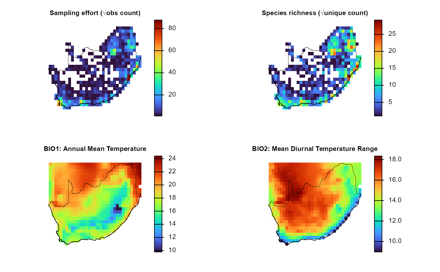
Bind climate, effort, and richness into one raster
stack: combines √-scaled effort (
obs_sum), √-scaled richness (spp_rich), and the 19 climate layers into a singleSpatRastaligned to the 0.5° grid. - Inspect the extracted covariates: produces a quick map (e.g. mean annual temperature) and previews the data to verify alignment and plausibility.
-
Assemble a modelling matrix: consolidates
coordinates, effort, richness, and all climate predictors into a tidy
data frame (
grid_env) ready for statistical modelling. -
Optional >> Reproject centroids for
metric-space analyses: converts centroid coordinates from
WGS-84(EPSG:4326) to aAlbers Equal-Areaprojection (EPSG:9822) when analyses require distances in metres.
Download and sample 19 WorldClim bioclim
variables
Fetch the 5-arc-min (~10 km) bioclim stack via geodata
package and attach values to every centroid.
# Retrieve 19 bioclim layers (≈10-km, WorldClim v2.1) for all grid centroids
data_path = system.file("extdata", package = "dissmapr")               # cache folder for rasters
enviro_list = dissmapr::get_enviro_data(
  data       = grid_spp,                  # centroids + obs_sum + spp_rich
  buffer_km  = 10,                        # pad the AOI slightly
  source     = "geodata",                 # WorldClim/SoilGrids interface
  var        = "bio",                     # bioclim variable set
  res        = 5,                         # 5-arc-min ≈ 10 km
  path       = data_path,
  sp_cols    = 7:ncol(grid_spp),          # ignore species columns
  ext_cols   = c("obs_sum", "spp_rich")   # carry effort & richness through
)

# Quick checks
str(enviro_list, max.level = 1)
#> List of 3
#>  $ env_rast:S4 class 'SpatRaster' [package "terra"]
#>  $ sites_sf: sf [415 × 2] (S3: sf/tbl_df/tbl/data.frame)
#>   ..- attr(*, "sf_column")= chr "geometry"
#>   ..- attr(*, "agr")= Factor w/ 3 levels "constant","aggregate",..: NA
#>   .. ..- attr(*, "names")= chr "grid_id"
#>  $ env_df  : tibble [415 × 24] (S3: tbl_df/tbl/data.frame)

# (Optional) Assign concise layer names for readability
# Find names here https://www.worldclim.org/data/bioclim.html
names_env = c("temp_mean","mdr","iso","temp_sea","temp_max","temp_min",
              "temp_range","temp_wetQ","temp_dryQ","temp_warmQ",
              "temp_coldQ","rain_mean","rain_wet","rain_dry",
              "rain_sea","rain_wetQ","rain_dryQ","rain_warmQ","rain_coldQ")
names(enviro_list$env_rast) = names_env

# (Optional) Promote frequently-used objects
env_r = enviro_list$env_rast    # cropped climate stack
env_df = enviro_list$env_df      # site × environment data-frame

# Quick checks
env_r
#> class       : SpatRaster
#> size        : 154, 195, 19  (nrow, ncol, nlyr)
#> resolution  : 0.08333333, 0.08333333  (x, y)
#> extent      : 16.66667, 32.91667, -34.91667, -22.08333  (xmin, xmax, ymin, ymax)
#> coord. ref. : lon/lat WGS 84 (EPSG:4326)
#> source(s)   : memory
#> names       : temp_mean,       mdr,       iso,   temp_sea,  temp_max, temp_min, ...
#> min values  :  5.158916,  5.891667, 45.320835,  143.07431,    14.832,   -6.284, ...
#> max values  : 24.796417, 18.659584, 67.097374, 701.333496, 38.518002,     13.8, ...
dim(env_df); head(env_df)
#> [1] 415  24
#> # A tibble: 6 × 24
#>   grid_id centroid_lon centroid_lat bio01 bio02 bio03 bio04 bio05 bio06 bio07
#>   <chr>          <dbl>        <dbl> <dbl> <dbl> <dbl> <dbl> <dbl> <dbl> <dbl>
#> 1 1026            28.8        -22.3  21.9  14.5  55.7  427.  32.4  6.44  26.0
#> 2 1027            29.2        -22.3  21.8  14.6  53.9  453.  33.0  5.87  27.1
#> 3 1028            29.7        -22.3  21.5  14.0  56.3  393.  31.7  6.80  24.9
#> 4 1029            30.3        -22.3  23.0  13.7  57.8  358.  32.8  9.14  23.7
#> 5 1030            30.8        -22.3  23.6  13.8  59.6  334.  33.5 10.3   23.2
#> 6 1031            31.3        -22.3  24.6  14.6  61.7  332.  34.8 11.0   23.8
#> # ℹ 14 more variables: bio08 <dbl>, bio09 <dbl>, bio10 <dbl>, bio11 <dbl>,
#> #   bio12 <dbl>, bio13 <dbl>, bio14 <dbl>, bio15 <dbl>, bio16 <dbl>,
#> #   bio17 <dbl>, bio18 <dbl>, bio19 <dbl>, obs_sum <dbl>, spp_rich <dbl>
get_enviro_data() buffered the grid centroids by 10
km, fetched the requested rasters, cropped them, extracted values at
each centroid, filled isolated NAs, and merged the results with
obs_sum and spp_rich.
2. Bind climate, effort, and richness into one raster stack
Fuse the √-scaled sampling‐effort (obs_sum) and richness
(spp_rich) layers with the 19 bioclim rasters
into a single, co-registered SpatRast. A unified stack
ensures that all predictors share the same grid, streamlining downstream
map algebra, multivariate modelling, and spatial cross-validation.
# --- Rebuild rasters inside the vignette ---
effRich_r = sqrt(
  grid_r[[c("obs_sum", "spp_rich")]]
)

# Use first layer as template explicitly
template = effRich_r[[1]]

env_resampled = terra::resample(
  env_r,
  template,
  method = "bilinear"
)

env_effRich_r = c(effRich_r, env_resampled)

# --- Safe plotting ---
old_par = par(no.readonly = TRUE)
on.exit(par(old_par), add = TRUE)

layout(matrix(1:4, nrow = 2))

titles = c(
  "Sampling effort (√obs count)",
  "Species richness (√unique count)",
  "BIO1: Annual Mean Temperature",
  "BIO2: Mean Diurnal Temperature Range"
)

for (i in 1:4) {
  terra::plot(
    env_effRich_r[[i]],
    col    = viridisLite::turbo(100),
    type   = "continuous",
    colNA  = NA_character_,
    axes   = FALSE,
    main   = titles[i],
    cex.main = 0.8
  )
  terra::plot(terra::vect(rsa), add = TRUE, border = "black", lwd = 0.4)
}
3. Inspect the extracted covariates
Environmental data were linked to grid centroids using
get_enviro_data(), now visualise the spatial variation in
selected climate variables to check results.
# Make column headers explicit
# names(env_df)[1:5] = c("grid_id","centroid_lon","centroid_lat","obs_sum","spp_rich")

# Simple check of dimensions and first rows
dim(env_df)
#> [1] 415  24
head(env_df[, 1:6])
#> # A tibble: 6 × 6
#>   grid_id centroid_lon centroid_lat bio01 bio02 bio03
#>   <chr>          <dbl>        <dbl> <dbl> <dbl> <dbl>
#> 1 1026            28.8        -22.3  21.9  14.5  55.7
#> 2 1027            29.2        -22.3  21.8  14.6  53.9
#> 3 1028            29.7        -22.3  21.5  14.0  56.3
#> 4 1029            30.3        -22.3  23.0  13.7  57.8
#> 5 1030            30.8        -22.3  23.6  13.8  59.6
#> 6 1031            31.3        -22.3  24.6  14.6  61.7

# Quick map of mean annual temperature (√-scaled bubble size)
ggplot() +
  geom_sf(data = grid_sf, fill = NA, colour = "darkgrey", alpha = 0.4) +
  geom_point(data = env_df,
             aes(x = centroid_lon,
                 y = centroid_lat,
                 colour = bio01),
             shape = 15,
             size = 3) +
  # scale_size_continuous(range = c(2,6)) +
  scale_colour_viridis_c(option = "turbo") +
  geom_sf(data = rsa, fill = NA, colour = "black") +
  theme_minimal() +
  labs(title = "Grid-cell mean annual temperature (√-scaled)",
       x = "Longitude", y = "Latitude")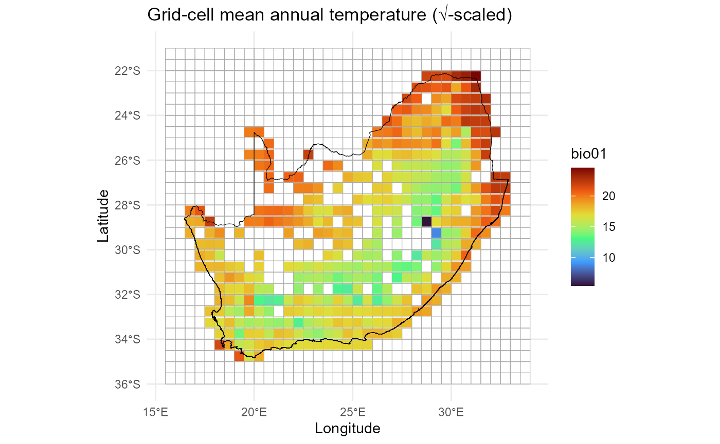
Goal of this plot is to quickly check that the environmental
predictors (e.g. bio01 >> mean annual temperature)
line up with the 0.5° grid.
4. Assemble the modelling matrix grid_env
Compile a site × environment data frame
(grid_env) in which each 0.5° cell contributes one row
containing centroid coordinates, √-scaled sampling effort, species
richness, and the 19 bioclim predictors. The resulting
matrix is immediately usable for GLMs, GAMs, machine-learning,
ordination, and β-diversity analyses.
# Build the final site × environment table
grid_env = env_df %>%
  dplyr::select(grid_id, centroid_lon, centroid_lat,
                obs_sum, spp_rich, dplyr::everything())

str(grid_env, max.level = 1)
#> tibble [415 × 24] (S3: tbl_df/tbl/data.frame)
head(grid_env)
#> # A tibble: 6 × 24
#>   grid_id centroid_lon centroid_lat obs_sum spp_rich bio01 bio02 bio03 bio04
#>   <chr>          <dbl>        <dbl>   <dbl>    <dbl> <dbl> <dbl> <dbl> <dbl>
#> 1 1026            28.8        -22.3       3        2  21.9  14.5  55.7  427.
#> 2 1027            29.2        -22.3      41       31  21.8  14.6  53.9  453.
#> 3 1028            29.7        -22.3      10       10  21.5  14.0  56.3  393.
#> 4 1029            30.3        -22.3       7        7  23.0  13.7  57.8  358.
#> 5 1030            30.8        -22.3       6        6  23.6  13.8  59.6  334.
#> 6 1031            31.3        -22.3     107       76  24.6  14.6  61.7  332.
#> # ℹ 15 more variables: bio05 <dbl>, bio06 <dbl>, bio07 <dbl>, bio08 <dbl>,
#> #   bio09 <dbl>, bio10 <dbl>, bio11 <dbl>, bio12 <dbl>, bio13 <dbl>,
#> #   bio14 <dbl>, bio15 <dbl>, bio16 <dbl>, bio17 <dbl>, bio18 <dbl>,
#> #   bio19 <dbl>
5. Reproject centroids for metric-space analyses** using
sf::st_transform()[OPTIONAL]
Certain analyses (e.g. spatial clustering, variogram modelling)
require coordinates in metres rather than degrees. The snippet below
converts the centroid layer to an Albers Equal-Area
projection.
# Convert the centroid columns to an sf object
centroids_sf = sf::st_as_sf(
  grid_env,
  coords = c("centroid_lon", "centroid_lat"),
  crs    = 4326,          # WGS-84
  remove = FALSE
)

# Reproject to Albers Equal Area (EPSG 9822)
centroids_aea = sf::st_transform(centroids_sf, 9822)

# Append projected X–Y back onto the data-frame
grid_env = cbind(
  grid_env,
  sf::st_coordinates(centroids_aea) |>
    as.data.frame() |>
    setNames(c("x_aea", "y_aea"))   # rename within the pipeline
)
names(grid_env)
#>  [1] "grid_id"      "centroid_lon" "centroid_lat" "obs_sum"      "spp_rich"
#>  [6] "bio01"        "bio02"        "bio03"        "bio04"        "bio05"
#> [11] "bio06"        "bio07"        "bio08"        "bio09"        "bio10"
#> [16] "bio11"        "bio12"        "bio13"        "bio14"        "bio15"
#> [21] "bio16"        "bio17"        "bio18"        "bio19"        "x_aea"
#> [26] "y_aea"
head(grid_env[, c("grid_id","centroid_lon","centroid_lat","x_aea","y_aea")])
#>   grid_id centroid_lon centroid_lat   x_aea    y_aea
#> 1    1026        28.75    -22.25004 6392274 -6836200
#> 2    1027        29.25    -22.25004 6480542 -6808542
#> 3    1028        29.75    -22.25004 6568648 -6780369
#> 4    1029        30.25    -22.25004 6656587 -6751682
#> 5    1030        30.75    -22.25004 6744357 -6722482
#> 6    1031        31.25    -22.25004 6831955 -6692770
At this point every grid cell has species metrics, climate predictors, and is optionally projected into metre coordinates, all in a single tidy object.
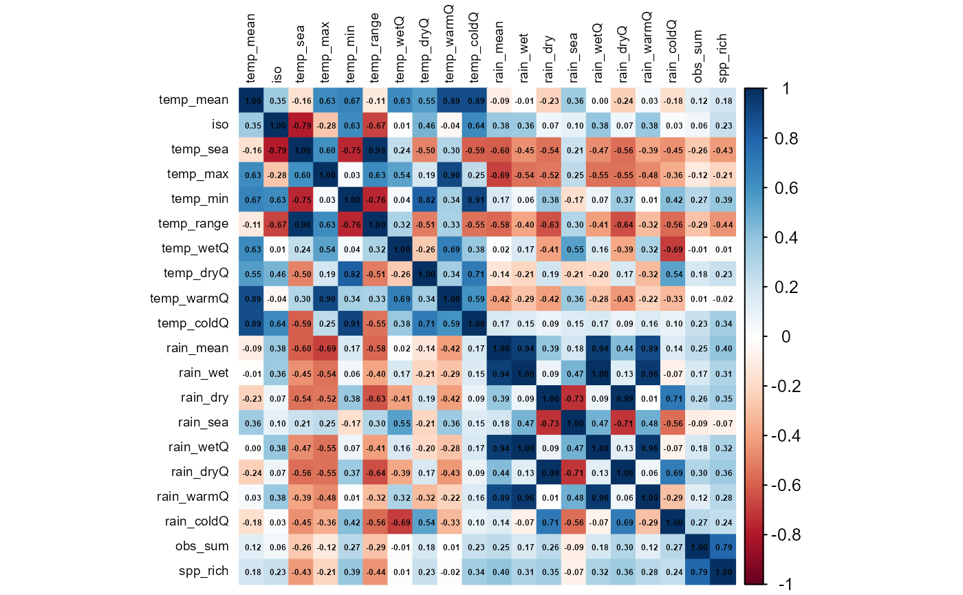
6. Diagnose and mitigate collinearity with
rm_correlated()
Highly inter-correlated predictors inflate variance, bias coefficient
estimates, and complicate ecological inference.rm_correlated() screens the environmental matrix for
pairwise correlations that exceed a user-defined threshold (here |r|
> 0.70), then iteratively prunes the variable with the highest
average absolute correlation. The routine
- Computes a Pearson (default) Correlation matrix for
the supplied columns;
-
Ranks variables by their mean absolute
correlation;
-
Discards the worst offender, recomputes the matrix,
and repeats until all remaining pairs lie below the threshold;
- Optional >> displays the final Correlation heat-map for visual QC.
The result is a reduced predictor set that retains maximal information while minimising multicollinearity.
# (Optional) Rename BIO
names(env_df) = c("grid_id", "centroid_lon", "centroid_lat", names_env, "obs_sum", "spp_rich")

# Run the filter and compare dimensions
# Filter environmental predictors for |r| > 0.70
env_vars_reduced = dissmapr::rm_correlated(
  data       = env_df[, c(4, 6:24)],  # drop ID + coord columns
  cols       = NULL,                  # infer all numeric cols
  threshold  = 0.70,
  plot       = TRUE                   # show heat-map of retained vars
)
# Before vs after
c(original = ncol(env_df[, c(4, 6:24)]),
  reduced  = ncol(env_vars_reduced))
#> original  reduced
#>       20        7
env_vars_reduced now contains a decorrelated subset
of climate predictors suitable for stable GLMs, GAMs, machine-learning,
or ordination workflows.
sessionInfo()
#> R version 4.5.2 (2025-10-31 ucrt)
#> Platform: x86_64-w64-mingw32/x64
#> Running under: Windows 11 x64 (build 26200)
#>
#> Matrix products: default
#>   LAPACK version 3.12.1
#>
#> locale:
#> [1] LC_COLLATE=English_South Africa.utf8  LC_CTYPE=English_South Africa.utf8
#> [3] LC_MONETARY=English_South Africa.utf8 LC_NUMERIC=C
#> [5] LC_TIME=English_South Africa.utf8
#>
#> time zone: Africa/Johannesburg
#> tzcode source: internal
#>
#> attached base packages:
#> [1] stats     graphics  grDevices datasets  utils     methods   base
#>
#> other attached packages:
#> [1] dplyr_1.2.1    ggplot2_4.0.3  dissmapr_0.2.0
#>
#> loaded via a namespace (and not attached):
#>   [1] DBI_1.3.0            pbapply_1.7-4        geodata_0.6-9
#>   [4] pROC_1.19.0.1        s2_1.1.11            permute_0.9-10
#>   [7] rlang_1.2.0          magrittr_2.0.5       otel_0.2.0
#>  [10] e1071_1.7-17         compiler_4.5.2       mgcv_1.9-4
#>  [13] systemfonts_1.3.2    vctrs_0.7.3          maps_3.4.3
#>  [16] reshape2_1.4.5       stringr_1.6.0        wk_0.9.5
#>  [19] pkgconfig_2.0.3      fastmap_1.2.0        labeling_0.4.3
#>  [22] utf8_1.2.6           rmarkdown_2.31       prodlim_2026.03.11
#>  [25] ragg_1.5.2           purrr_1.2.2          xfun_0.59
#>  [28] cachem_1.1.0         jsonlite_2.0.0       recipes_1.3.3
#>  [31] terra_1.9-34         parallel_4.5.2       cluster_2.1.8.2
#>  [34] R6_2.6.1             bslib_0.11.0         stringi_1.8.7
#>  [37] RColorBrewer_1.1-3   parallelly_1.47.0    rpart_4.1.27
#>  [40] estimability_1.5.1   lubridate_1.9.5      jquerylib_0.1.4
#>  [43] Rcpp_1.1.1-1.1       iterators_1.0.14     knitr_1.51
#>  [46] future.apply_1.20.2  fields_17.3          zoo_1.8-15
#>  [49] Matrix_1.7-5         splines_4.5.2        nnet_7.3-20
#>  [52] timechange_0.4.0     tidyselect_1.2.1     rstudioapi_0.19.0
#>  [55] yaml_2.3.12          vegan_2.7-5          timeDate_4052.112
#>  [58] codetools_0.2-20     listenv_1.0.0        lattice_0.22-9
#>  [61] tibble_3.3.1         plyr_1.8.9           withr_3.0.3
#>  [64] S7_0.2.2             geosphere_1.6-8      evaluate_1.0.5
#>  [67] sf_1.1-1             future_1.70.0        desc_1.4.3
#>  [70] survival_3.8-6       units_1.0-1          proxy_0.4-29
#>  [73] mclust_6.1.2         pillar_1.11.1        KernSmooth_2.23-26
#>  [76] corrplot_0.95        renv_1.1.4           foreach_1.5.2
#>  [79] stats4_4.5.2         generics_0.1.4       zetadiv_1.3.0
#>  [82] scales_1.4.0         xtable_1.8-8         globals_0.19.1
#>  [85] class_7.3-23         glue_1.8.1           clValid_0.7
#>  [88] emmeans_2.0.3        tools_4.5.2          data.table_1.18.4
#>  [91] ModelMetrics_1.2.2.2 gower_1.0.2          mvtnorm_1.4-1
#>  [94] fs_2.1.0             dotCall64_1.2        grid_4.5.2
#>  [97] tidyr_1.3.2          ipred_0.9-15         nlme_3.1-169
#> [100] patchwork_1.3.2      cli_3.6.6            rappdirs_0.3.4
#> [103] textshaping_1.0.5    NbClust_3.0.1        spam_2.11-4
#> [106] viridisLite_0.4.3    scam_1.2-22          lava_1.9.1
#> [109] gtable_0.3.6         sass_0.4.10          digest_0.6.39
#> [112] classInt_0.4-11      caret_7.0-1          ggrepel_0.9.8
#> [115] htmlwidgets_1.6.4    farver_2.1.2         entropy_1.3.2
#> [118] htmltools_0.5.9      pkgdown_2.2.0        lifecycle_1.0.5
#> [121] factoextra_2.0.0     hardhat_1.4.3        httr_1.4.8
#> [124] MASS_7.3-65