Calculate Biodiversity Indicators Over Space

This function provides a flexible framework for calculating various biodiversity indicators on a spatial grid or as a time series. It prepares the data, creates a grid, calculates indicators, and formats the output into an appropriate S3 object ('indicator_map'). Specific implementations for different indicator types are provided using the appropriate wrappers.

Usage

# S3 method for class 'obs_richness'
calc_map(x, ...)

# S3 method for class 'total_occ'
calc_map(x, ...)

# S3 method for class 'newness'
calc_map(x, newness_min_year = NULL, ...)

# S3 method for class 'occ_density'
calc_map(x, ...)

# S3 method for class 'williams_evenness'
calc_map(x, ...)

# S3 method for class 'pielou_evenness'
calc_map(x, ...)

# S3 method for class 'ab_rarity'
calc_map(x, ...)

# S3 method for class 'area_rarity'
calc_map(x, ...)

# S3 method for class 'spec_occ'
calc_map(x, ...)

# S3 method for class 'spec_range'
calc_map(x, ...)

# S3 method for class 'tax_distinct'
calc_map(x, ...)

calc_map(x, ...)

Arguments

x

A data cube object ('processed_cube').

...

Additional arguments passed to specific indicator calculation functions.

newness_min_year

If set, only shows values above this (e.g. 1970). Values below the minimum will be replaced with NA. This can be useful e.g. if you have outlier cells where the data is very old causing the legend gradient to stretch in a way that makes other cell values difficult to discern.

Value

An S3 object of the class 'indicator_map' containing the calculated indicator values and metadata.

Examples

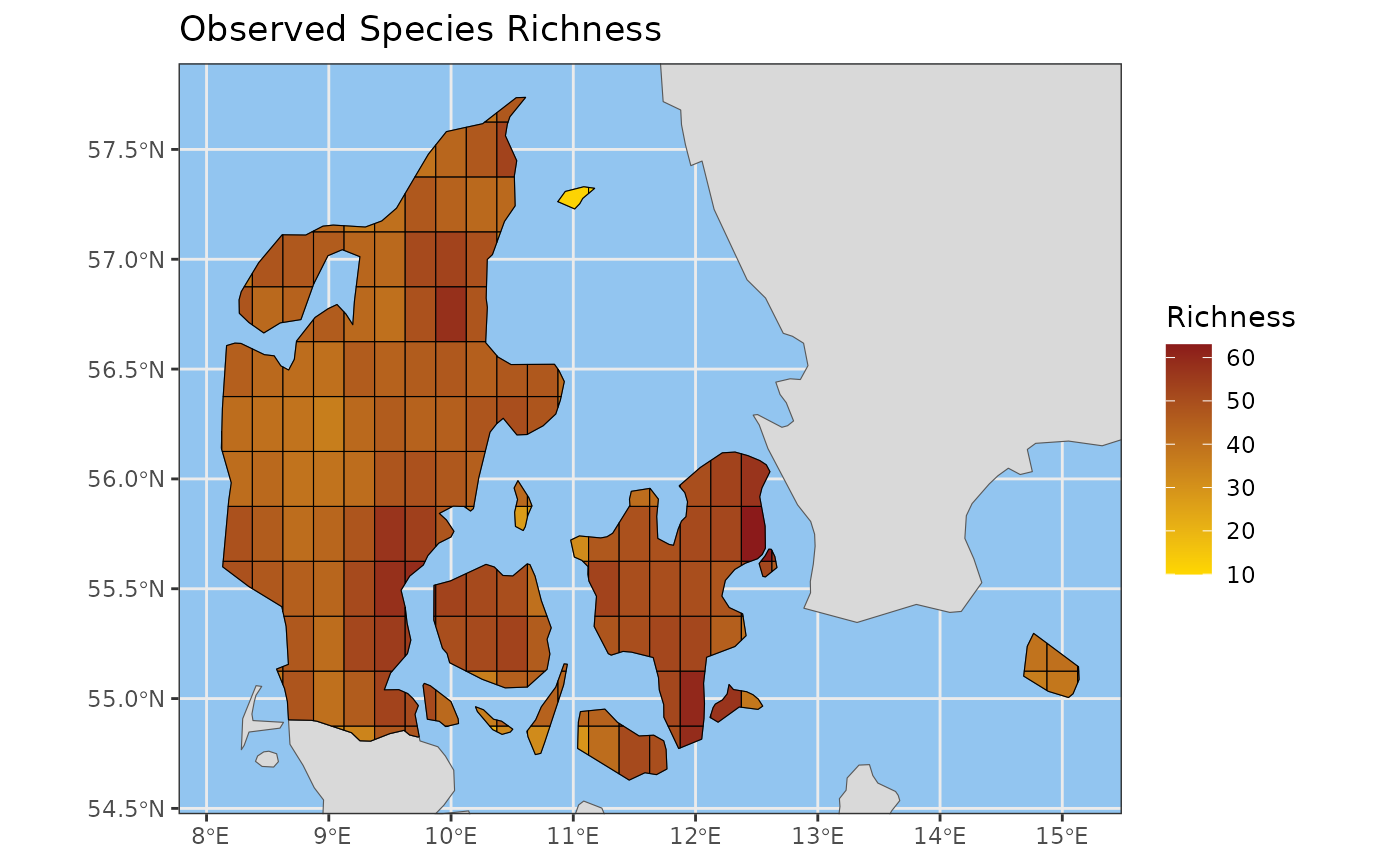
observed_richness_map <- obs_richness_map(example_cube_1, level = "country", region = "Denmark")
plot(observed_richness_map)