A Gentle Introduction to b3gbi: Data Cubes to Biodiversity Indicators

Introduction

The goal of the b3gbi package (B3 General Biodiversity Indicators) is to provide standardized, automated, and reproducible workflows for calculating essential spatial and temporal biodiversity indicators. Developed as part of the EU-funded B3 (Biodiversity Building Blocks for Policy) project, b3gbi takes pre-processed GBIF occurrence cubes as input and quickly transforms them into actionable metrics, including richness, evenness, rarity, taxonomic distinctness, Shannon-Hill diversity, Simpson-Hill diversity, and completeness, complete with integrated uncertainty estimation using robust bootstrapping methods.

This tutorial will guide you through the three core steps of the b3gbi workflow:

Data Ingestion: Preparing your GBIF data cube with process_cube().
Indicator Calculation: Using indicator-specific wrapper functions.
Visualization: Plotting the results as maps or time series using the generic plot() function.

The package is publicly available at https://www.github.com/b-cubed-eu/b3gbi.

Package Installation

The package is available on the dedicated B-Cubed R-universe repository.

# Install the package from the dedicated R-universe
install.packages("b3gbi", repos = "https://b-cubed-eu.r-universe.dev")

# Load the package
library(b3gbi)

Step 1: Data Ingestion with `process_cube()`

The first step is importing your GBIF occurrence cube (a .csv file) and converting it into a structured processed_cube object. This function automatically validates the input and attempts to autodetect column names and grid types.

Key `process_cube()` Arguments

Argument	Description	Default/Details
`data`	Path to the .csv file containing the GBIF cube. Required.
`grid_type`	The grid system used (e.g., ‘eea’, ‘mgrs’, ‘eqdgc’, ‘isea3h’, ‘custom’).	Autodetected if possible.
`first_year`	Filters the cube to start at this year.	First year in the data.
`last_year`	Filters the cube to end at this year.	Last year in the data.

Note on Column Names: The function automatically attempts to detect required columns (like cell code, year, species key). You only need to manually specify arguments like cols_year or cols_cellCode if your column names deviate from expected standards.

Example: Import Data and Filter by Time

Here we import an example cube of mammals in Denmark, filtering the data to start from 1980.

# Function 1: process_cube()
denmark_cube <- process_cube(
  system.file("extdata",
    "denmark_mammals_cube_eqdgc.csv",
    package = "b3gbi"
  ),
  first_year = 1980
) # Filter the cube to start at 1980

# Printing the object shows key metadata
denmark_cube
#> 
#> Processed data cube for calculating biodiversity indicators
#> 
#> Date Range: 1980 - 2024 
#> Single-resolution cube with cell size 0.25degrees 
#> Number of cells: 186 
#> Grid reference system: eqdgc 
#> Coordinate range:
#>  xmin  xmax  ymin  ymax 
#>  3.75 15.25 54.50 58.25 
#> 
#> Total number of observations: 6064 
#> Number of species represented: 53 
#> Number of families represented: 19 
#> 
#> Kingdoms represented: Animalia 
#> 
#> First 10 rows of data (use n = to show more):
#> 
#> # A tibble: 969 × 15
#>     year cellCode  kingdomKey kingdom  familyKey family  taxonKey scientificName
#>    <dbl> <chr>     <chr>      <chr>    <chr>     <chr>   <chr>    <chr>         
#>  1  1980 E010N55AA 1          Animalia 5307      Mustel… 5219019  Mustela ermin…
#>  2  1980 E012N55AD 1          Animalia 5534      Sorici… 8316400  Sorex araneus 
#>  3  1981 E008N55CB 1          Animalia 5310      Phocid… 2434806  Halichoerus g…
#>  4  1981 E010N57BA 1          Animalia 3240723   Cricet… 4265185  Arvicola amph…
#>  5  1981 E011N57CC 1          Animalia 5310      Phocid… 2434806  Halichoerus g…
#>  6  1982 E010N56AD 1          Animalia 5310      Phocid… 2434806  Halichoerus g…
#>  7  1982 E011N56DC 1          Animalia 5310      Phocid… 2434793  Phoca vitulina
#>  8  1983 E009N55CD 1          Animalia 9379      Lepori… 7952072  Lepus europae…
#>  9  1983 E011N55AB 1          Animalia 5310      Phocid… 2434793  Phoca vitulina
#> 10  1983 E015N55CA 1          Animalia 5310      Phocid… 2434806  Halichoerus g…
#> # ℹ 959 more rows
#> # ℹ 7 more variables: obs <dbl>, minCoordinateUncertaintyInMeters <dbl>,
#> #   minTemporalUncertainty <dbl>, familyCount <dbl>, xcoord <dbl>,
#> #   ycoord <dbl>, resolution <chr>

The data itself is stored in a tibble within the object’s data slot, and the rest is metadata.

str(denmark_cube)
#> List of 11
#>  $ first_year  : num 1980
#>  $ last_year   : num 2024
#>  $ coord_range :List of 4
#>   ..$ xmin: num 3.75
#>   ..$ xmax: num 15.2
#>   ..$ ymin: num 54.5
#>   ..$ ymax: num 58.2
#>  $ num_cells   : int 186
#>  $ num_species : int 53
#>  $ num_obs     : num 6064
#>  $ kingdoms    : chr "Animalia"
#>  $ num_families: int 19
#>  $ grid_type   : chr "eqdgc"
#>  $ resolutions : chr "0.25degrees"
#>  $ data        : tibble [969 × 15] (S3: tbl_df/tbl/data.frame)
#>   ..$ year                            : num [1:969] 1980 1980 1981 1981 1981 ...
#>   ..$ cellCode                        : chr [1:969] "E010N55AA" "E012N55AD" "E008N55CB" "E010N57BA" ...
#>   ..$ kingdomKey                      : chr [1:969] "1" "1" "1" "1" ...
#>   ..$ kingdom                         : chr [1:969] "Animalia" "Animalia" "Animalia" "Animalia" ...
#>   ..$ familyKey                       : chr [1:969] "5307" "5534" "5310" "3240723" ...
#>   ..$ family                          : chr [1:969] "Mustelidae" "Soricidae" "Phocidae" "Cricetidae" ...
#>   ..$ taxonKey                        : chr [1:969] "5219019" "8316400" "2434806" "4265185" ...
#>   ..$ scientificName                  : chr [1:969] "Mustela erminea" "Sorex araneus" "Halichoerus grypus" "Arvicola amphibius" ...
#>   ..$ obs                             : num [1:969] 1 1 3 1 1 1 1 1 2 2 ...
#>   ..$ minCoordinateUncertaintyInMeters: num [1:969] 930 390 3 870 3 3 3 780 3 3 ...
#>   ..$ minTemporalUncertainty          : num [1:969] 86400 86400 86400 86400 86400 86400 86400 86400 86400 86400 ...
#>   ..$ familyCount                     : num [1:969] 23427 1360 39284 1954 39284 ...
#>   ..$ xcoord                          : num [1:969] 10.12 12.38 8.38 10.62 11.12 ...
#>   ..$ ycoord                          : num [1:969] 55.9 55.6 55.4 57.9 57.1 ...
#>   ..$ resolution                      : chr [1:969] "0.25degrees" "0.25degrees" "0.25degrees" "0.25degrees" ...
#>  - attr(*, "class")= chr "processed_cube"

Step 2: Indicator Calculation

The package provides numerous wrappers to calculate indicators as either maps (spatial distribution) or time series (temporal trends).

Available Indicators

Use available_indicators to see the full list of indicators and their associated wrapper functions (e.g., obs_richness_map, total_occ_ts).

available_indicators
#> 
#> 
#> Available Indicators
#> 
#> 
#> 1. Observed Species Richness
#>     Class: obs_richness
#>     Calculate map: yes, e.g. obs_richness_map(my_data_cube)
#>     Calculate time series: yes, e.g. obs_richness_ts(my_data_cube)
#>     Additional map function arguments: NA
#>     Additional time series function arguments: NA
#> 
#> 2. Total Occurrences
#>     Class: total_occ
#>     Calculate map: yes, e.g. total_occ_map(my_data_cube)
#>     Calculate time series: yes, e.g. total_occ_ts(my_data_cube)
#>     Additional map function arguments: NA
#>     Additional time series function arguments: NA
#> 
#> 3. Pielou's Evenness
#>     Class: pielou_evenness
#>     Calculate map: yes, e.g. pielou_evenness_map(my_data_cube)
#>     Calculate time series: yes, e.g. pielou_evenness_ts(my_data_cube)
#>     Additional map function arguments: NA
#>     Additional time series function arguments: NA
#> 
#> 4. Williams' Evenness
#>     Class: williams_evenness
#>     Calculate map: yes, e.g. williams_evenness_map(my_data_cube)
#>     Calculate time series: yes, e.g. williams_evenness_ts(my_data_cube)
#>     Additional map function arguments: NA
#>     Additional time series function arguments: NA
#> 
#> 5. Cumulative Species Richness
#>     Class: cum_richness
#>     Calculate map: no
#>     Calculate time series: yes, e.g. cum_richness_ts(my_data_cube)
#>     Additional map function arguments: NA
#>     Additional time series function arguments: NA
#> 
#> 6. Density of Occurrences
#>     Class: occ_density
#>     Calculate map: yes, e.g. occ_density_map(my_data_cube)
#>     Calculate time series: yes, e.g. occ_density_ts(my_data_cube)
#>     Additional map function arguments: NA
#>     Additional time series function arguments: NA
#> 
#> 7. Abundance-Based Rarity
#>     Class: ab_rarity
#>     Calculate map: yes, e.g. ab_rarity_map(my_data_cube)
#>     Calculate time series: yes, e.g. ab_rarity_ts(my_data_cube)
#>     Additional map function arguments: NA
#>     Additional time series function arguments: NA
#> 
#> 8. Area-Based Rarity
#>     Class: area_rarity
#>     Calculate map: yes, e.g. area_rarity_map(my_data_cube)
#>     Calculate time series: yes, e.g. area_rarity_ts(my_data_cube)
#>     Additional map function arguments: NA
#>     Additional time series function arguments: NA
#> 
#> 9. Mean Year of Occurrence
#>     Class: newness
#>     Calculate map: yes, e.g. newness_map(my_data_cube)
#>     Calculate time series: yes, e.g. newness_ts(my_data_cube)
#>     Additional map function arguments: NA
#>     Additional time series function arguments: NA
#> 
#> 10. Taxonomic Distinctness
#>     Class: tax_distinct
#>     Calculate map: yes, e.g. tax_distinct_map(my_data_cube)
#>     Calculate time series: yes, e.g. tax_distinct_ts(my_data_cube)
#>     Additional map function arguments: rows
#>     Additional time series function arguments: rows
#> 
#> 11. Species Richness (Estimated by Coverage-Based Rarefaction)
#>     Class: hill0
#>     Calculate map: yes, e.g. hill0_map(my_data_cube)
#>     Calculate time series: yes, e.g. hill0_ts(my_data_cube)
#>     Additional map function arguments: cutoff_length, coverage, conf_level, data_type, assume_freq
#>     Additional time series function arguments: cutoff_length, coverage, conf_level, data_type, assume_freq
#> 
#> 12. Hill-Shannon Diversity (Estimated by Coverage-Based Rarefaction)
#>     Class: hill1
#>     Calculate map: yes, e.g. hill1_map(my_data_cube)
#>     Calculate time series: yes, e.g. hill1_ts(my_data_cube)
#>     Additional map function arguments: cutoff_length, coverage, conf_level, data_type, assume_freq
#>     Additional time series function arguments: cutoff_length, coverage, conf_level, data_type, assume_freq
#> 
#> 13. Hill-Simpson Diversity (Estimated by Coverage-Based Rarefaction)
#>     Class: hill2
#>     Calculate map: yes, e.g. hill2_map(my_data_cube)
#>     Calculate time series: yes, e.g. hill2_ts(my_data_cube)
#>     Additional map function arguments: cutoff_length, coverage, conf_level, data_type, assume_freq
#>     Additional time series function arguments: cutoff_length, coverage, conf_level, data_type, assume_freq
#> 
#> 14. Species Occurrences
#>     Class: spec_occ
#>     Calculate map: yes, e.g. spec_occ_map(my_data_cube)
#>     Calculate time series: yes, e.g. spec_occ_ts(my_data_cube)
#>     Additional map function arguments: NA
#>     Additional time series function arguments: NA
#> 
#> 15. Species Range
#>     Class: spec_range
#>     Calculate map: yes, e.g. spec_range_map(my_data_cube)
#>     Calculate time series: yes, e.g. spec_range_ts(my_data_cube)
#>     Additional map function arguments: NA
#>     Additional time series function arguments: NA
#> 
#> 16. Occupancy Turnover
#>     Class: occ_turnover
#>     Calculate map: no
#>     Calculate time series: yes, e.g. occ_turnover_ts(my_data_cube)
#>     Additional map function arguments: NA
#>     Additional time series function arguments: NA
#> 
#> 17. Species Richness Density
#>     Class: spec_richness_density
#>     Calculate map: yes, e.g. spec_richness_density_map(my_data_cube)
#>     Calculate time series: yes, e.g. spec_richness_density_ts(my_data_cube)
#>     Additional map function arguments: NA
#>     Additional time series function arguments: NA
#> 
#> 18. Completeness (Sample Coverage)
#>     Class: completeness
#>     Calculate map: yes, e.g. completeness_map(my_data_cube)
#>     Calculate time series: yes, e.g. completeness_ts(my_data_cube)
#>     Additional map function arguments: cutoff_length, data_type, assume_freq
#>     Additional time series function arguments: cutoff_length, data_type, assume_freq, gridded_average
#> 
#> 19. Species Relative Occupancy
#>     Class: relative_occupancy
#>     Calculate map: yes, e.g. relative_occupancy_map(my_data_cube)
#>     Calculate time series: yes, e.g. relative_occupancy_ts(my_data_cube)
#>     Additional map function arguments: NA
#>     Additional time series function arguments: NA

Core Arguments for Wrapper Functions

All indicator wrapper functions (e.g., obs_richness_map, occ_turnover_ts) share the following key arguments:

Argument	Description	Details
`data`	The `processed_cube` object. Required.
`level`	The geographical scale (‘country’, ‘continent’, ‘world’).	Automatically retrieves boundaries.
`region`	The specific region name (e.g., ‘Germany’, ‘Europe’).	Required if level is set.

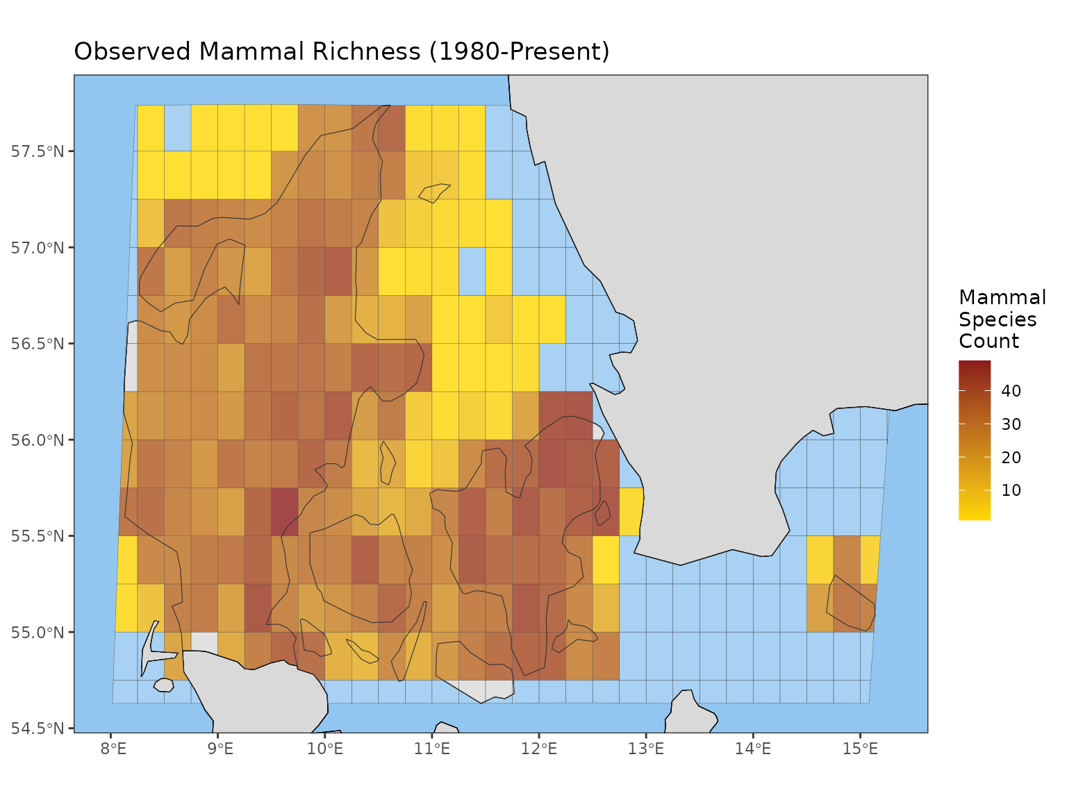
Example: Observed Species Richness Map

Let’s calculate the observed richness spatially, covering the period from 1980 to the end of the cube’s data.

# Calculate a gridded map of observed species richness for Denmark
# Note that confidence intervals are not calculated for map indicators
Denmark_observed_richness_map <- obs_richness_map(denmark_cube, 
                                                   level = "country", 
                                                   region = "Denmark")

The result is an indicator_map object (the data within it is also an sf object, containing geographical information).

class(Denmark_observed_richness_map)
#> [1] "indicator_map" "obs_richness"
class(Denmark_observed_richness_map$data)
#> [1] "indicator_data" "sf"             "tbl_df"         "tbl"           
#> [5] "data.frame"

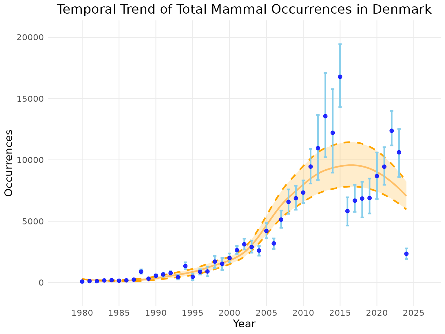
Example: Total Occurrences Time Series

Now, let’s calculate the same indicator temporally for a trend analysis.

# Calculate a time series of total occurrences for Denmark
# By default, confidence intervals are NOT calculated during this step
Denmark_total_occ_ts <- total_occ_ts(denmark_cube, 
                                     level = "country", 
                                     region = "Denmark")

The result is an indicator_ts object.

class(Denmark_total_occ_ts)
#> [1] "indicator_ts" "total_occ"

Now let’s add confidence intervals using the add_ci() function. To speed things up we will reduce the number of bootstrap samples from the default of 1000 to 100. By default, the package uses percentile intervals ("perc"), which are robust for biodiversity indicators.

# Add confidence intervals to the time series
Denmark_total_occ_ts_with_ci <- add_ci(Denmark_total_occ_ts, 
                                       num_bootstrap = 100)
#> [1] "Performing group-specific bootstrap with `boot::boot()`."

For more in-depth information on how uncertainty is handled, the different types of confidence intervals available, and advanced configuration options, please see the Uncertainty in Biodiversity Indicators vignette.

Step 3: Visualization with `plot()`

The generic plot() function automatically calls the appropriate helper function (plot_map() or plot_ts()) and applies smart defaults for titles, colors, and layout.

Plotting the Map

Argument	Description	Common Use
`title`	Sets the plot title.	e.g., “Observed Richness in Denmark”
`legend_title`	Sets the legend title.	e.g., “Number of Species”
`crop_to_grid`	If TRUE, the map edges are determined by the grid extent.
`crop_by_region`	If TRUE, map edges are determined by the map region selected during indicator calculation, rather than the data.

# Plotting the map object
plot(Denmark_observed_richness_map,
  legend_title = "Mammal Species Count",
  title = "Observed Mammal Richness (1980-Present)"
)

Plotting the Time Series

If your indicator_ts object contains confidence intervals, the plot() function will automatically display them as ribbons or error bars.

# Plotting the time series object
plot(Denmark_total_occ_ts,
  title = "Temporal Trend of Total Mammal Occurrences in Denmark",
  linecolour = "blue",
  ribboncolour = "skyblue",
  trendlinecolour = "darkorange",
  envelopecolour = "orange",
  smoothed_trend = TRUE
)

Shawn Dove