Bootstrap Method for Data Cubes

Introduction

When working with data cubes, it’s essential to understand the uncertainty surrounding derived statistics. This tutorial introduces the bootstrap_cube() function from dubicube, which uses bootstrap resampling to estimate the variability, bias, and standard error of estimates.

Bootstrapping for data cubes

Bootstrapping is a resampling method used to approximate the distribution of a statistic by repeatedly sampling from the data with replacement. In the context of biodiversity data cubes, bootstrap_cube() enables us to assess the variability of derived statistics, such as by computing confidence intervals.

A data cube and a statistic

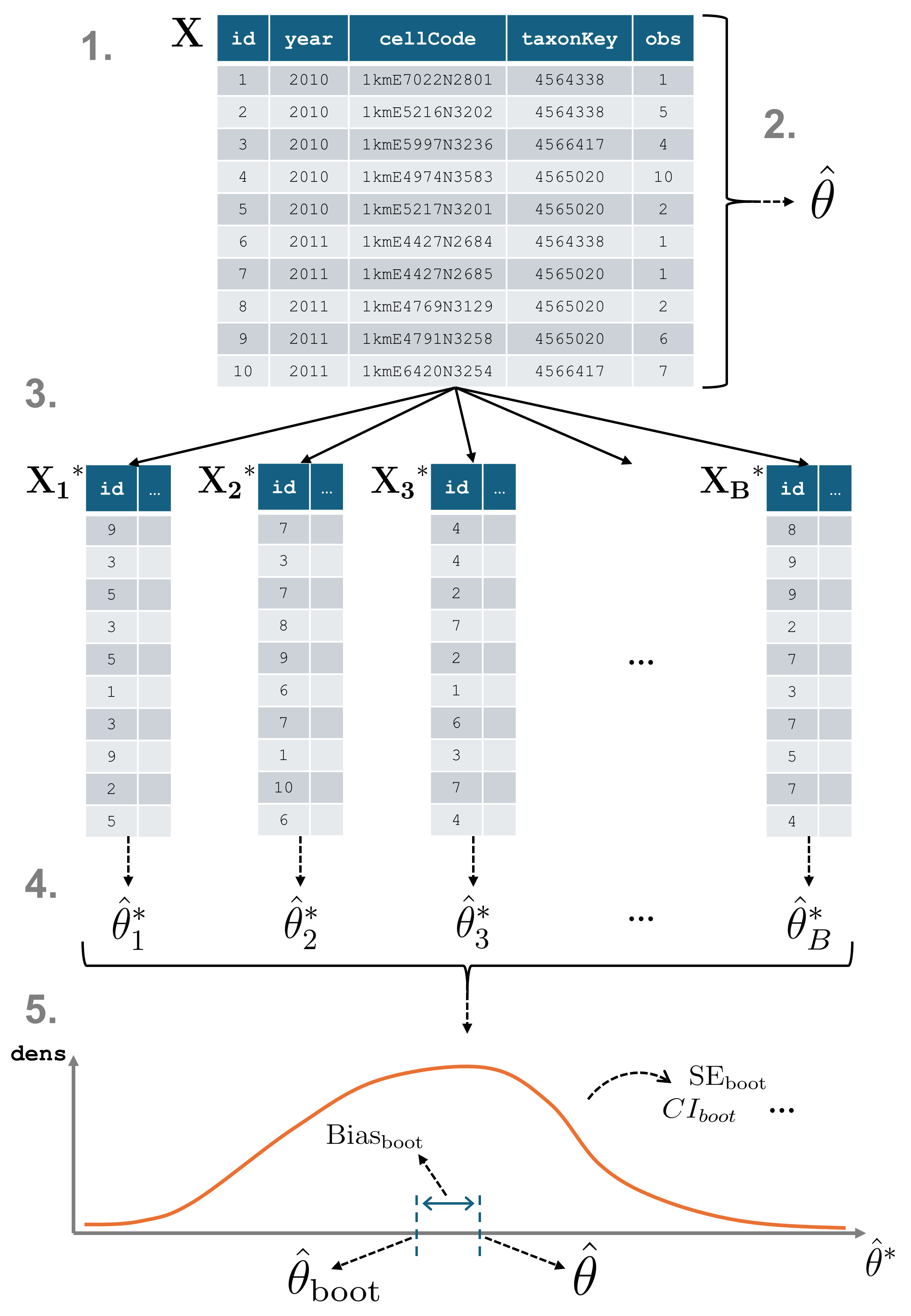
Consider a data cube $\mathbf{X}$ from which we want to calculate a statistic $\theta$.

Original Sample Data: $\mathbf{X} = \{X_1, X_2, \ldots, X_n\}$
- The initial set of data points. Here, $n$ is the sample size. This corresponds to the number of cells in a data cube or the number of rows in tabular format.
Statistic of Interest: $\theta$
- The parameter or statistic being estimated, such as the mean $\bar{X}$, variance $\sigma^2$, or a biodiversity indicator. Let $\hat{\theta}$ denote the estimated value of $\theta$ calculated from the complete dataset $\mathbf{X}$.

Resampling and recalculating

From $\mathbf{X}$, multiple resampled datasets $\mathbf{X}^*$ are created by sampling rows (cells) with replacement until each new dataset is equally large as $\mathbf{X}$. This process is repeated $B$ times, and each resample yields a new estimate $\hat{\theta}^*_b$ of the statistic.

Bootstrap Sample: $\mathbf{X}^* = \{X_1^*, X_2^*, \ldots, X_n^*\}$
- A sample of size $n$ drawn with replacement from the original sample $\mathbf{X}$. Each $X_i^*$ is drawn independently from $\mathbf{X}$.
- A total of $B$ bootstrap samples are drawn from the original data. Common choices for $B$ are 1000 or 10,000 to ensure a good approximation of the distribution of the bootstrap replications (see further).
Bootstrap Replication: $\hat{\theta}^*_b$
- The value of the statistic of interest calculated from the $b$-th bootstrap sample $\mathbf{X}^*_b$. For example, if $\theta$ is the sample mean, $\hat{\theta}^*_b = \bar{X}^*_b$.

Derivation of bootstrap statistics

The set of bootstrap replications forms the bootstrap distribution, which can be used to estimate bootstrap statistics and construct confidence intervals (see the interval calculation tutorial).

Bootstrap Estimate of the Statistic: $\hat{\theta}_{\text{boot}}$
- The average of the bootstrap replications:

\[ \hat{\theta}_{\text{boot}} = \frac{1}{B} \sum_{b=1}^B \hat{\theta}^*_b \]

Bootstrap Bias: $\text{Bias}_{\text{boot}}$
- This bias indicates how much the bootstrap estimate deviates from the original sample estimate. It is calculated as the difference between the average bootstrap estimate and the original estimate:

\[ \text{Bias}_{\text{boot}} = \frac{1}{B} \sum_{b=1}^B (\hat{\theta}^*_b - \hat{\theta}) = \hat{\theta}_{\text{boot}} - \hat{\theta} \]

Bootstrap Standard Error: $\text{SE}_{\text{boot}}$
- The standard deviation of the bootstrap replications, which estimates the variability of the statistic.

Bootstrap resampling a data cube.

Getting started with dubicube

Our method can be used on any dataframe from which a statistic is calculated and a grouping variable is present. For this tutorial, we focus on occurrence cubes. Therefore, we will use the b3gbi package for processing the raw data before we go over to bootstrapping.

# Load packages
library(dubicube)

# Data loading and processing
library(frictionless) # Load example datasets
library(b3gbi)        # Process occurrence cubes

# General
library(ggplot2)      # Data visualisation
library(dplyr)        # Data wrangling
library(tidyr)        # Data wrangling

Loading and processing the data

We load the bird cube data from the b3data data package using frictionless (see also here). It is an occurrence cube for birds in Belgium between 2000 en 2024 using the MGRS grid at 10 km scale.

# Read data package
b3data_package <- read_package(
  "https://zenodo.org/records/15211029/files/datapackage.json"
)

# Load bird cube data
bird_cube_belgium <- read_resource(b3data_package, "bird_cube_belgium_mgrs10")
head(bird_cube_belgium)
#> # A tibble: 6 × 8
#>    year mgrscode specieskey species          family     n mincoordinateuncerta…¹
#>   <dbl> <chr>         <dbl> <chr>            <chr>  <dbl>                  <dbl>
#> 1  2000 31UDS65     2473958 Perdix perdix    Phasi…     1                   3536
#> 2  2000 31UDS65     2474156 Coturnix coturn… Phasi…     1                   3536
#> 3  2000 31UDS65     2474377 Fulica atra      Ralli…     5                   1000
#> 4  2000 31UDS65     2475443 Merops apiaster  Merop…     6                   1000
#> 5  2000 31UDS65     2480242 Vanellus vanell… Chara…     1                   3536
#> 6  2000 31UDS65     2480637 Accipiter nisus  Accip…     1                   3536
#> # ℹ abbreviated name: ¹mincoordinateuncertaintyinmeters
#> # ℹ 1 more variable: familycount <dbl>

We process the cube with b3gbi. First, we select 2000 random rows to make the dataset smaller. This is to reduce the computation time for this tutorial. We select the data from 2011 - 2020.

set.seed(123)

# Make dataset smaller
rows <- sample(nrow(bird_cube_belgium), 2000)
bird_cube_belgium <- bird_cube_belgium[rows, ]

# Process cube
processed_cube <- process_cube(
  bird_cube_belgium,
  first_year = 2011,
  last_year = 2020,
  cols_occurrences = "n"
)
processed_cube
#> 
#> Processed data cube for calculating biodiversity indicators
#> 
#> Date Range: 2011 - 2020 
#> Single-resolution cube with cell size 10km ^2 
#> Number of cells: 242 
#> Grid reference system: mgrs 
#> Coordinate range:
#>    xmin    xmax    ymin    ymax 
#>  280000  710000 5490000 5700000 
#> 
#> Total number of observations: 45143 
#> Number of species represented: 253 
#> Number of families represented: 57 
#> 
#> Kingdoms represented: Data not present 
#> 
#> First 10 rows of data (use n = to show more):
#> 
#> # A tibble: 957 × 13
#>     year cellCode taxonKey scientificName    family   obs minCoordinateUncerta…¹
#>    <dbl> <chr>       <dbl> <chr>             <chr>  <dbl>                  <dbl>
#>  1  2011 31UFS56   5231918 Cuculus canorus   Cucul…    11                   3536
#>  2  2011 31UES28   5739317 Phoenicurus phoe… Musci…     6                   3536
#>  3  2011 31UFS64   6065824 Chroicocephalus … Larid…   143                   1000
#>  4  2011 31UFS96   2492576 Muscicapa striata Musci…     3                   3536
#>  5  2011 31UES04   5231198 Passer montanus   Passe…     1                   3536
#>  6  2011 31UES85   5229493 Garrulus glandar… Corvi…    23                    707
#>  7  2011 31UES88  10124612 Anser anser x Br… Anati…     1                    100
#>  8  2011 31UES22   2481172 Larus marinus     Larid…     8                   1000
#>  9  2011 31UFS43   2481139 Larus argentatus  Larid…    10                   3536
#> 10  2011 31UFT00   9274012 Spatula querqued… Anati…     8                   3536
#> # ℹ 947 more rows
#> # ℹ abbreviated name: ¹minCoordinateUncertaintyInMeters
#> # ℹ 6 more variables: familyCount <dbl>, xcoord <dbl>, ycoord <dbl>,
#> #   utmzone <int>, hemisphere <chr>, resolution <chr>

Analysis of the data

Let’s say we are interested in the mean number of observations per grid cell per year. We create a function to calculate this.

# Function to calculate statistic of interest
# Mean observations per grid cell per year
mean_obs <- function(data) {
  obs <- x <- NULL

  data %>%
    dplyr::mutate(x = mean(obs), .by = "cellCode") %>%
    dplyr::summarise(diversity_val = mean(x), .by = "year") %>%
    as.data.frame()
}

We get the following results:

mean_obs(processed_cube$data)
#>    year diversity_val
#> 1  2011      34.17777
#> 2  2012      35.27201
#> 3  2013      33.25581
#> 4  2014      55.44160
#> 5  2015      49.24754
#> 6  2016      48.34063
#> 7  2017      70.42202
#> 8  2018      48.83850
#> 9  2019      47.46795
#> 10 2020      43.00411

On their own, these values don’t reveal how much uncertainty surrounds them. To better understand their variability, we use bootstrapping to estimate the distribution of the yearly means.

Bootstrapping

We use the bootstrap_cube() function to do this. It relies on the following arguments:

data_cube:
The input data as a processed data cube (from b3gbi::process_cube()).
fun:
A user-defined function that computes the statistic(s) of interest from data_cube$data. This function should return a dataframe that includes a column named diversity_val, containing the statistic to evaluate.
grouping_var:
The column(s) used for grouping the output of fun(). For example, if fun() returns one value per year, use grouping_var = "year".
samples:
The number of bootstrap samples to draw. Common values are 1000 or more for reliable estimates of variability and confidence intervals.
seed:
An optional numeric seed to ensure reproducibility of the bootstrap resampling. Set this to a fixed value to get consistent results across runs.
progress:
Logical flag to show a progress bar. Set to TRUE to enable progress reporting; default is FALSE.

bootstrap_results <- bootstrap_cube(
  data_cube = processed_cube,
  fun = mean_obs,
  grouping_var = "year",
  samples = 1000,
  seed = 123
)

head(bootstrap_results)
#>   sample year est_original rep_boot est_boot se_boot  bias_boot
#> 1      1 2011     34.17777 24.23133 33.80046 4.24489 -0.3773142
#> 2      2 2011     34.17777 24.28965 33.80046 4.24489 -0.3773142
#> 3      3 2011     34.17777 31.81445 33.80046 4.24489 -0.3773142
#> 4      4 2011     34.17777 33.42530 33.80046 4.24489 -0.3773142
#> 5      5 2011     34.17777 35.03502 33.80046 4.24489 -0.3773142
#> 6      6 2011     34.17777 33.72037 33.80046 4.24489 -0.3773142

We can visualise the bootstrap distributions using a violin plot.

# Get bias vales
bias_mean_obs <- bootstrap_results %>%
  distinct(year, estimate = est_original, `bootstrap estimate` = est_boot)

# Get estimate values
estimate_mean_obs <- bias_mean_obs %>%
  pivot_longer(cols = c("estimate", "bootstrap estimate"),
               names_to = "Legend", values_to = "value") %>%
  mutate(Legend = factor(Legend, levels = c("estimate", "bootstrap estimate"),
                         ordered = TRUE))

# Visualise bootrap distributions
bootstrap_results %>%
  ggplot(aes(x = year)) +
  # Distribution
  geom_violin(aes(y = rep_boot, group = year),
              fill = alpha("cornflowerblue", 0.2)) +
  # Estimates and bias
  geom_point(data = estimate_mean_obs, aes(y = value, shape = Legend),
             colour = "firebrick", size = 2.5) +
  # Settings
  labs(y = "Mean Number of Observations\nper Grid Cell",
       x = "", shape = "Legend:") +
  scale_x_continuous(breaks = sort(unique(bootstrap_results$year))) +
  theme_minimal() +
  theme(legend.position = "bottom",
        legend.title = element_text(face = "bold"))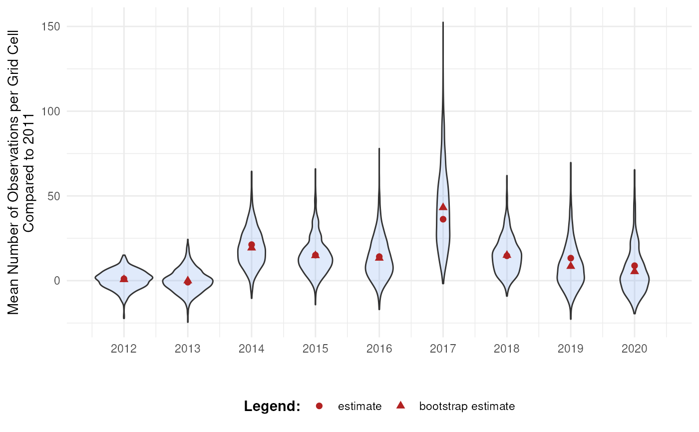

Bootstrap distributions for mean number of occurrences over time.

Advanced usage of `bootstrap_cube()`

Bootstrap simple dataframes

As stated in the documentation, it is also possible to bootstrap a dataframe. In this case, set the argument processed_cube = FALSE. This is implemented allow for flexible use of simple dataframes, while still encouraging the use of b3gbi::process_cube() as default functionality.

bootstrap_results_df <- bootstrap_cube(
  data_cube = processed_cube$data,      # data.frame object
  fun = mean_obs,
  grouping_var = "year",
  samples = 1000,
  seed = 123,
  processed_cube = FALSE
)

Comparison with a reference group

A particularly insightful approach is comparing indicator values to a reference group. In time series analyses, this often means comparing each year’s indicator to a baseline year (e.g., the first or last year in the series).

To do this, we perform bootstrapping over the difference between indicator values:

Resample the dataset with replacement
Calculate the indicator for each group (e.g., each year)
For each non-reference group, compute the difference between its indicator value and that of the reference group
Repeat steps 1–3 across all bootstrap iterations

This process yields bootstrap replicate distributions of differences in indicator values.

bootstrap_results_ref <- bootstrap_cube(
  data_cube = processed_cube,
  fun = mean_obs,
  grouping_var = "year",
  samples = 1000,
  ref_group = 2011,
  seed = 123
)

head(bootstrap_results_ref)
#>   sample year est_original   rep_boot  est_boot  se_boot  bias_boot
#> 1      1 2012     1.094245  8.1881078 0.6583191 5.475053 -0.4359261
#> 2      2 2012     1.094245  7.6061946 0.6583191 5.475053 -0.4359261
#> 3      3 2012     1.094245 -4.6058908 0.6583191 5.475053 -0.4359261
#> 4      4 2012     1.094245  2.4102039 0.6583191 5.475053 -0.4359261
#> 5      5 2012     1.094245  6.2626545 0.6583191 5.475053 -0.4359261
#> 6      6 2012     1.094245 -0.1577162 0.6583191 5.475053 -0.4359261

We see that the mean number of observations is higher in most years compared to 2011. At what point can we say these differences are significant? This will be further explored in the effect classification tutorial.

# Get bias vales
bias_mean_obs <- bootstrap_results_ref %>%
  distinct(year, estimate = est_original, `bootstrap estimate` = est_boot)

# Get estimate values
estimate_mean_obs <- bias_mean_obs %>%
  pivot_longer(cols = c("estimate", "bootstrap estimate"),
               names_to = "Legend", values_to = "value") %>%
  mutate(Legend = factor(Legend, levels = c("estimate", "bootstrap estimate"),
                         ordered = TRUE))

# Visualise bootrap distributions
bootstrap_results_ref %>%
  ggplot(aes(x = year)) +
  # Distribution
  geom_violin(aes(y = rep_boot, group = year),
              fill = alpha("cornflowerblue", 0.2)) +
  # Estimates and bias
  geom_point(data = estimate_mean_obs, aes(y = value, shape = Legend),
             colour = "firebrick", size = 2) +
  # Settings
  labs(y = "Mean Number of Observations per Grid Cell\nCompared to 2011",
       x = "", shape = "Legend:") +
  scale_x_continuous(breaks = sort(unique(bootstrap_results_ref$year))) +
  theme_minimal() +
  theme(legend.position = "bottom",
        legend.title = element_text(face = "bold"))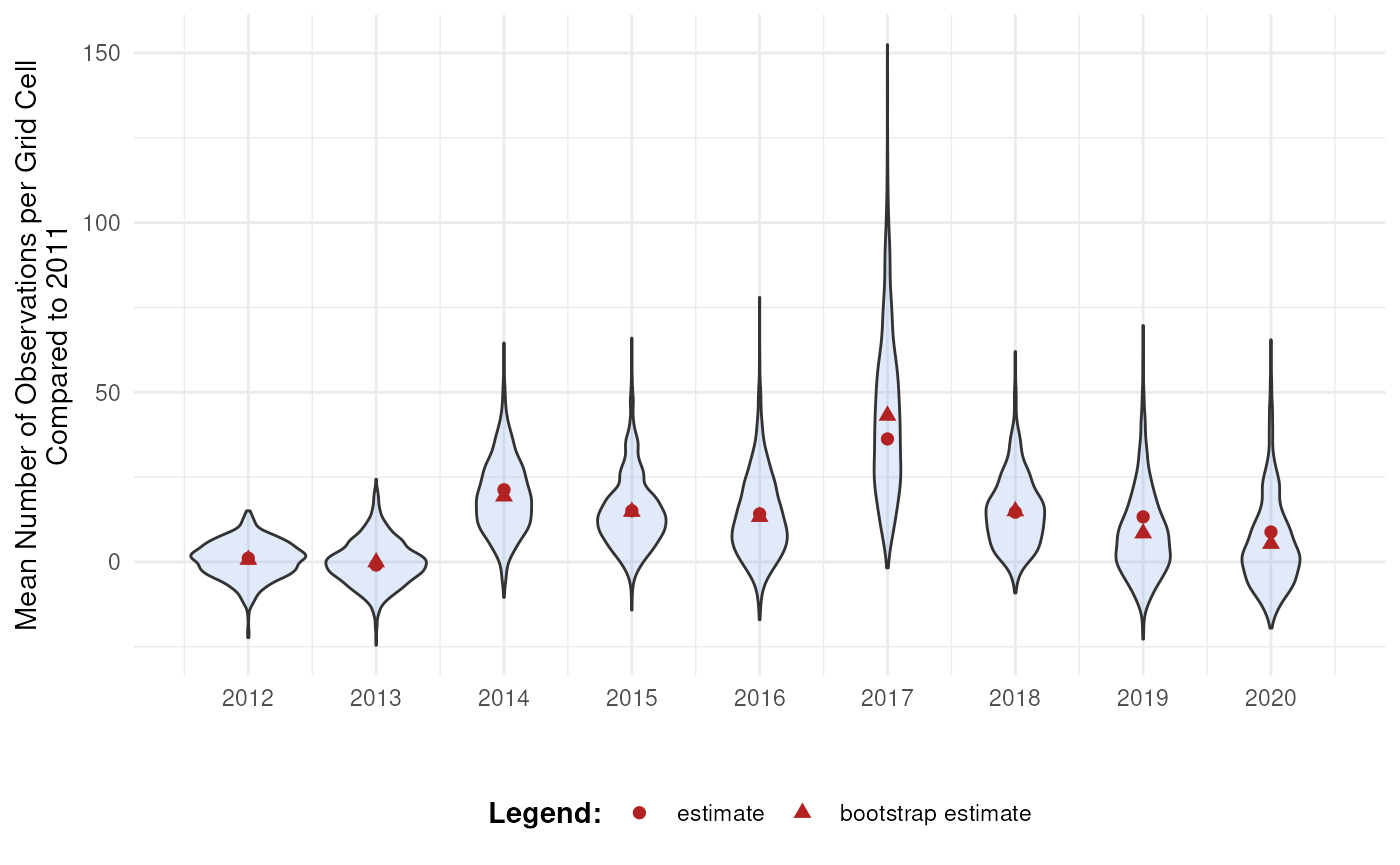

Bootstrap distributions for mean number of occurrences over time (ref).

Note that the choice of the reference year should be well considered. Keep in mind which comparisons should be made, and what the motivation is behind the reference period. A high or low value in the reference period relative to other periods, e.g. an exceptional bad or good year, can affect the magnitude and direction of the calculated differences. Whether this should be avoided or not, depends on the motivation behind the choice and the research question. A reference period can be determined by legislation, or by the start of a monitoring campaign. A specific research question can determine the periods that need to be compared. Furthermore, the variability of the estimate of reference period affects the width of confidence intervals for the differences. A more variable reference period will propagate greater uncertainty. In the case of GBIF data, more data will be available in recent years than in earlier years. If this is the case, it could make sense to select the last period as a reference period. In a way, this also avoids the arbitrariness of choice for the reference period. You compare previous situations with the current situation (last year), where you could repeat this comparison annually, for example. Finally, when comparing multiple indicators, we recommend using a consistent reference period to maintain comparability