Calculate Rarity Over Time or Space

This function calculates area-based or abundance-based rarity over a gridded map or as a time series (see 'Details' for more information).

Usage

area_rarity_map(data, ...)

area_rarity_ts(data, ...)

ab_rarity_map(data, ...)

ab_rarity_ts(data, ...)

Arguments

data

A data cube object (class 'processed_cube').

...

Arguments passed on to compute_indicator_workflow

cell_size

(Optional) Length of grid cell sides, in km or degrees. Only used for maps and for time series that require a grid.

"grid" (default): use the native resolution of the cube. If this would produce more than about 1 million grid cells over the study area (for degree-based cubes: if the resolution is finer than 1 degree for 'world' or 'continent', or finer than 0.1 degrees otherwise), you are asked to confirm in an interactive session, and the function stops with an error in a non-interactive session.
"auto": determined automatically. For km-based grids it depends on the area of the study region: 100 km for areas of at least 1 million sq km, 10 km for at least 10,000 sq km, 1 km for at least 100 sq km, and 0.1 km for smaller areas. For degree-based grids it is 1 degree for 'world' or 'continent' and 0.1 degrees otherwise. The automatic size is never smaller than the cube's resolution.
A number (in the units of the cube's resolution, i.e. km or degrees), or for km-based grids a string such as "10km" or "500m".

A manually selected cell size must be a whole number multiple of the cube's resolution.

level

(Optional) Spatial level: 'cube', 'continent', 'country', 'world', 'sovereignty', or 'geounit'. (Default: 'cube')

region

(Optional) The region of interest (e.g., "Denmark"). Ignored if level is 'cube' or 'world'. (Default: "Europe")

ne_type

(Optional) The type of Natural Earth data to download: 'countries', 'map_units', 'sovereignty', or 'tiny_countries'. This parameter is ignored if level is set to 'cube' or 'world'. (Default: "countries")

ne_scale

(Optional) The scale of Natural Earth data to download: 'small' - 110m, 'medium' - 50m, or 'large' - 10m. (Default: "medium")

output_crs

(Optional) The CRS you want for your calculated indicator. (Leave blank to let the function choose a default based on grid reference system.)

first_year

(Optional) Exclude data before this year. (Uses all data in the cube by default.)

last_year

(Optional) Exclude data after this year. (Uses all data in the cube by default.)

spherical_geometry

(Optional) If set to FALSE, will temporarily disable spherical geometry while the function runs. Should only be used to solve specific issues. (Default is TRUE).

make_valid

(Optional) Calls st_make_valid() from the sf package after creating the grid. Increases processing time but may help if you are getting polygon errors. (Default is FALSE).

shapefile_path

(optional) Path of an external shapefile to merge into the workflow. For example, if you want to calculate your indicator for particular features such as protected areas or wetlands.

shapefile_crs

(Optional) CRS of a .wkt shapefile. If your shapefile is .wkt and you do NOT use this parameter, the CRS will be assumed to be EPSG:4326 and the coordinates will be read in as lat/long. If your shape is NOT a .wkt the CRS will be determined automatically.

invert

(optional) Calculate an indicator over the inverse of the shapefile (e.g. if you have a protected areas shapefile this would calculate an indicator over all non protected areas within your cube). Default is FALSE.

include_land

(Optional) Include occurrences which fall within the land area. Default is TRUE. Note that this is purely a geographic filter, and does not filter based on whether the occurrence is actually terrestrial. Grid cells which fall partially on land and partially on ocean will be included even if include_land is FALSE. To exclude terrestrial and/or freshwater taxa, you must manually filter your data cube before calculating your indicator.

include_ocean

(Optional) Include occurrences which fall outside the land area. Default is TRUE. Set as "buffered_coast" to include a set buffer size around the land area rather than the entire ocean area. Note that this is purely a geographic filter, and does not filter based on whether the occurrence is actually marine. Grid cells which fall partially on land and partially on ocean will be included even if include_ocean is FALSE. To exclude marine taxa, you must manually filter your data cube before calculating your indicator.

buffer_dist_km

(Optional) The distance to buffer around the land if include_ocean is set to "buffered_coast". Default is 50 km.

force_grid

(Optional) Forces the calculation of a grid even if this would not normally be part of the pipeline, i.e. for time series. A grid is needed for time series of area-based rarity, Hill diversity and relative occupancy (and for completeness with gridded_average = TRUE). This is switched on automatically for these indicators: the wrappers area_rarity_ts(), hill0_ts(), hill1_ts() and hill2_ts() already set force_grid = TRUE, so do not pass it to them. (Default: FALSE)

Value

An S3 object with the classes 'indicator_map' or 'indicator_ts' and 'area_rarity' or 'ab_rarity' containing the calculated indicator values and metadata.

Details

Rarity

Rarity is the scarcity or infrequency of a particular species in an area. A rare species might have a small population size, a limited distribution, or a unique ecological niche (Maciel, 2021; Rabinowitz, 1981). Rarity can also be a biodiversity indicator when summed over multiple species in an area, and may provide important insight for determining conservation priorities. When measured over time, rarity may indicate potential threats or changes in the environment.

Abundance-Based Rarity

Abundance-based rarity is the inverse of the proportion of total occurrences represented by a particular species. The total summed rarity for each grid cell or year is calculated (sum the rarity values of each species present there). It is calculated as:

$$ \sum_{i=1}^{S} \frac{1}{p_i} $$

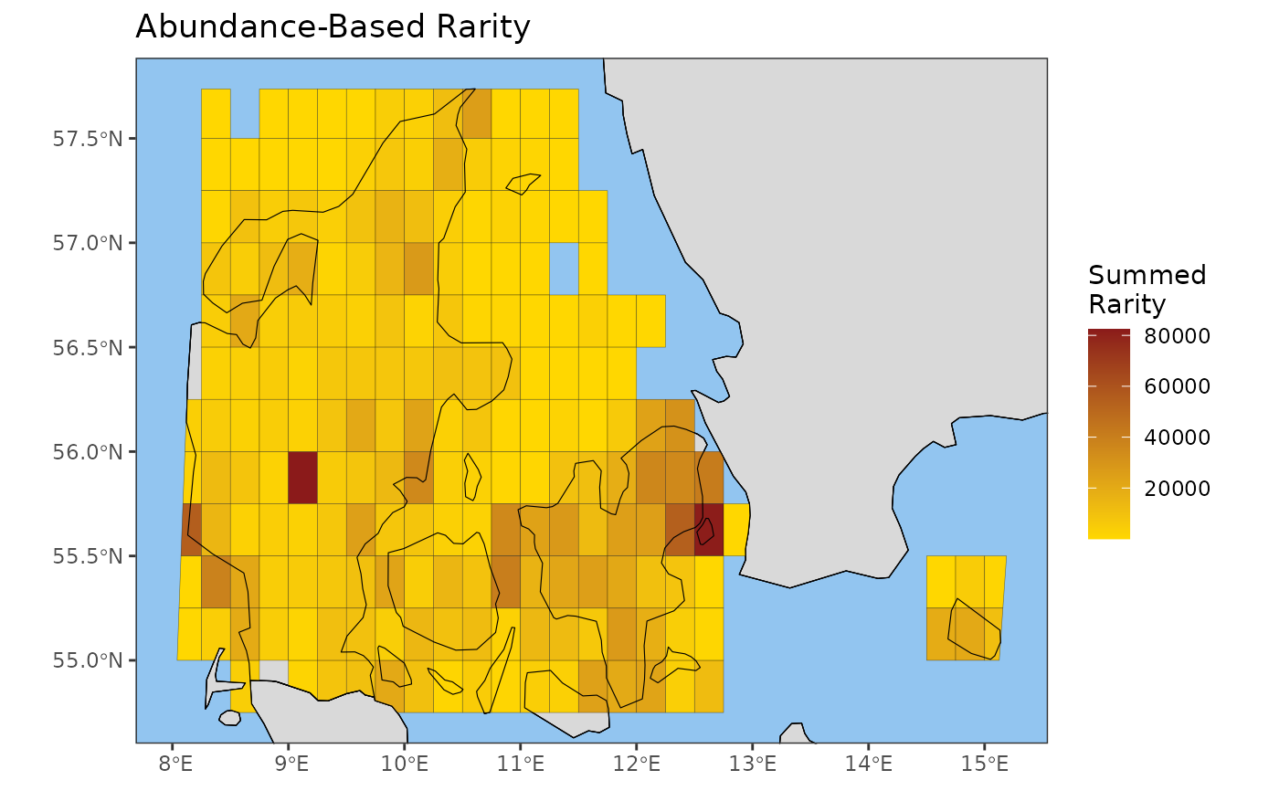
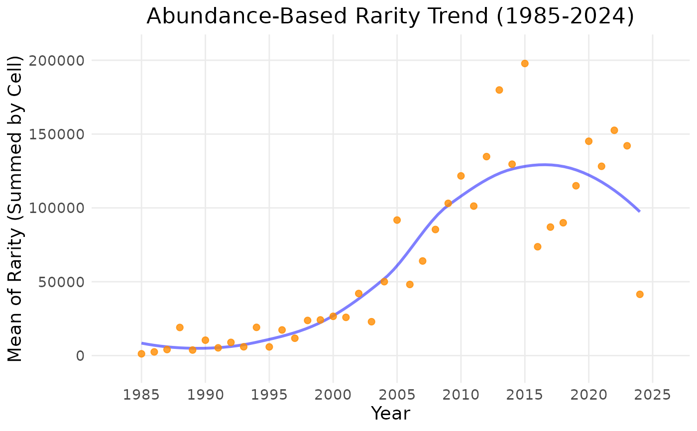
where S is the number of species and pi is the proportion of occurrences represented by species i. For maps, pi is calculated within each grid cell (over the whole time period). For time series, pi is calculated separately for each year (species i's occurrences that year divided by all occurrences that year), and each species present in a year contributes once.

Area-Based Rarity

Area-based rarity is the inverse of occupancy frequency (the proportion of occupied grid cells in which the species occurs) for a particular species. The total summed rarity for each grid cell or year is calculated (sum the rarity values of each species present there). It is calculated as:

$$ \sum_{i=1}^{S} \frac{N}{n_i} $$

where S is the number of species, N is the total number of occupied grid cells, and ni is the number of grid cells occupied by species i.

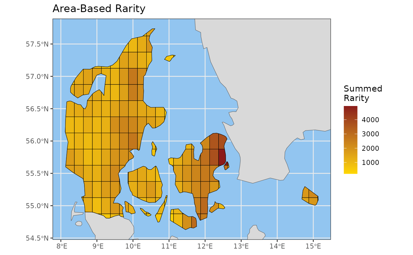
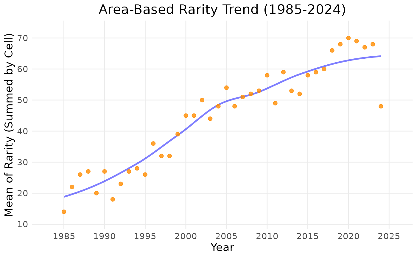
For maps, N and ni are calculated over the whole time period, and the summed rarity is reported for each grid cell. For time series, N and ni are calculated separately for each year; rarity is summed within each occupied grid cell and the yearly value is the mean of these cell sums.

Functions

area_rarity_map():
area_rarity_ts():
ab_rarity_map():
ab_rarity_ts():

References

Maciel, E. A. (2021). An index for assessing the rare species of a community. Ecological Indicators, 124, 107424.

Rabinowitz, D. (1981). Seven forms of rarity. *Biological aspects of rare * plant conservation.

Examples

# \donttest{
arr_map <- area_rarity_map(example_cube_1,
  level = "country",
  region = "Denmark"
)
plot(arr_map)

# }
# \donttest{
arr_ts <- area_rarity_ts(example_cube_1, first_year = 1985)
#> although coordinates are longitude/latitude, st_intersection assumes that they
#> are planar
plot(arr_ts)

# }
# \donttest{
abr_map <- ab_rarity_map(example_cube_1,
  level = "country",
  region = "Denmark"
)
plot(abr_map)

# }
# \donttest{
abr_ts <- ab_rarity_ts(example_cube_1, first_year = 1985)
plot(abr_ts)

# }