Simulate timeseries for species occurrences

This function simulates a timeseries for the number of occurrences of a species.

Usage

simulate_timeseries(
  initial_average_occurrences = 50,
  n_time_points = 1,
  temporal_function = NA,
  ...,
  seed = NA
)

Arguments

initial_average_occurrences: A positive numeric value indicating the average number of occurrences to be simulated at the first time point. This value serves as the mean (lambda) of a Poisson distribution.
n_time_points: A positive integer specifying the number of time points to simulate.
temporal_function: A function generating a trend in number of occurrences over time, or NA (default). If n_time_points > 1 and a function is provided, it defines the temporal pattern of number of occurrences.
...: Additional arguments to be passed to temporal_function.
seed: A positive numeric value setting the seed for random number generation to ensure reproducibility. If NA (default), then set.seed() is not called at all. If not NA, then the random number generator state is reset (to the state before calling this function) upon exiting this function.

Value

A vector of integers of length n_time_points with the number of occurrences.

Examples

# 1. Use the function simulate_random_walk()
simulate_timeseries(
  initial_average_occurrences = 50,
  n_time_points = 10,
  temporal_function = simulate_random_walk,
  sd_step = 1,
  seed = 123
)
#>  [1] 46 52 66 54 52 43 56 38 46 43

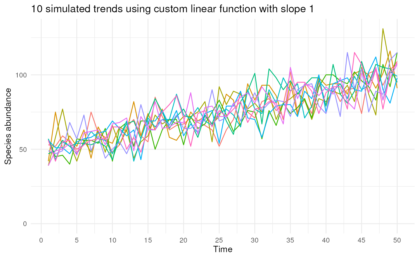
# 2. Using your own custom function, e.g. this linear function
my_own_linear_function <- function(
    initial_average_occurrences = initial_average_occurrences,
    n_time_points = n_time_points,
    coef) {
  # Calculate new average abundances over time
  time <- seq_len(n_time_points) - 1
  lambdas <- initial_average_occurrences + (coef * time)

  # Identify where the lambda values become 0 or lower
  zero_or_lower_index <- which(lambdas <= 0)

  # If any lambda becomes 0 or lower, set all subsequent lambdas to 0
  if (length(zero_or_lower_index) > 0) {
    zero_or_lower_indices <- zero_or_lower_index[1]:n_time_points
    lambdas[zero_or_lower_indices] <- 0
  }

  # Return average abundances
  return(lambdas)
}

# Draw n_sim number of occurrences from Poisson distribution using
# the custom function
n_sim <- 10
n_time_points <- 50
slope <- 1
list_abundances <- vector("list", length = n_sim)

# Loop n_sim times over simulate_timeseries()
for (i in seq_len(n_sim)) {
  abundances <- simulate_timeseries(
    initial_average_occurrences = 50,
    n_time_points = n_time_points,
    temporal_function = my_own_linear_function,
    coef = slope
  )

  list_abundances[[i]] <- data.frame(
    time = seq_along(abundances),
    abundance = abundances,
    sim = i
  )
}

# Combine list of dataframes
data_abundances <- do.call(rbind.data.frame, list_abundances)

# Plot the simulated abundances over time using ggplot2
library(ggplot2)
ggplot(data_abundances, aes(x = time, y = abundance, colour = factor(sim))) +
  geom_line() +
  labs(
    x = "Time", y = "Species abundance",
    title = paste(
      n_sim, "simulated trends using custom linear function",
      "with slope", slope
    )
  ) +
  scale_y_continuous(limits = c(0, NA)) +
  scale_x_continuous(breaks = seq(0, n_time_points, 5)) +
  theme_minimal() +
  theme(legend.position = "")

Usage

Arguments

Value

See also

Examples