Code
library(readr)
library(here)
library(dplyr)
library(patchwork)
library(tidyr)
library(purrr)
library(tibble)
library(trias)
library(countrycode)This document shows how using GBIF species occurrence cubes to assess the emerging status of raccoon (Procyon lotor) in Europe and in European countries. This workflow is strongly based on the occurrence TrIAS indicators and can be extended to other (invasive alien) species.
First, list and load the needed packages.
library(readr)
library(here)
library(dplyr)
library(patchwork)
library(tidyr)
library(purrr)
library(tibble)
library(trias)
library(countrycode)The species of interest is the raccoon (Procyon lotor (Linnaeus, 1758), GBIF Key: 5218786). This workflow can easily be extended to other species.
species <- tibble::tibble(
  specieskey = c(5218786),
  canonical_name = c("Procyon lotor")
)We are interested over the emerging status of the four species in the European countries and all Europe.
We request a species occurrence cube based on data from 1950.
We triggered a GBIF occurrence cube via the Occurrence SQL Download API and on the hand of a JSON query (query_cube_raccoon.json). The resulting cube (DOI: 10.15468/dl.mmnusj, downloadKey: 0023024-250127130748423) can be downloaded in TSV format from GBIF. We have it saved at data/input as 0023024-250127130748423.csv:
cube <- readr::read_tsv(
  here::here(
    "data",
    "input",
    "0023024-250127130748423.csv"
  )
)
Preview:
head(cube)Notice the presence of column countrycode as we grouped by country. It can happen that an occurrence is assigned to a cell in another country or a cell on the border of two different countries It happens few times:
cube |>
  dplyr::distinct(eeacellcode, countrycode, year) |>
  dplyr::add_count(eeacellcode, year) |>
  dplyr::filter(n > 1) |>
  dplyr::arrange(eeacellcode)
Countries with at least one occurrence:
cube |>
  dplyr::distinct(countrycode) |>
  dplyr::pull(countrycode)
[1] "BE" "NL" "DE" "AZ" "ES" "GB" "FR" "LU" "CH" "DK" "LI" "SE" "CZ" "AT" "PL"
[16] "RU" "GE" "IT" "LT" "IE" "UA" "PT" "NO"Remove countries not completely covered by the EEA grid:
UA)RU)AZ)cube <- cube |>
dplyr::filter(!countrycode %in% c("UA", "RU", "AZ"))Are there rows without eeacellcode?
cube |>
  dplyr::filter(is.na(eeacellcode))
We remove them:
cube <- cube |>
  dplyr::filter(!is.na(eeacellcode))
Extract country codes:
countrycode <- cube |>
  dplyr::distinct(countrycode) |>
  dplyr::pull(countrycode)
countrycode
[1] "BE" "NL" "DE" "ES" "GB" "FR" "LU" "CH" "DK" "LI" "SE" "CZ" "AT" "PL" "IT"
[16] "LT" "IE" "PT" "NO"Get country names from country codes:
countries <- tibble::tibble(
  countrycode = countrycode) |>
  dplyr::mutate(country_name = countrycode::countrycode(countrycode, "iso2c", "country.name"))
countries
We add "Europe" to the list of country names and codes. We use "Europe" as “country code”: the abbreviation EU would be confusing as it is the acronym of the European Union:
countries <- countries |>
  dplyr::add_row(countrycode = "Europe", country_name = "Europe")
countrycode <- c(countrycode, "Europe")
So, from now on, when we refer to “country”, we also mean “Europe”.
We calculate the cube for Europe:
cube_europe <- cube |>
  group_by(specieskey, species, year, eeacellcode) |>
  summarise(
    countrycode = "Europe",
    occurrences = sum(occurrences),
    class = unique(class),
    classkey = unique(classkey),
    mincoordinateuncertaintyinmeters = min(mincoordinateuncertaintyinmeters),
    mintemporaluncertainty = min(mintemporaluncertainty),
    classcount = unique(classcount),
    .groups = "drop") %>%
  # order columns as in the original cube
  dplyr::select(
    dplyr::all_of(names(cube))
  )
head(cube_europe)
And we add it to cube:
cube <- dplyr::bind_rows(cube, cube_europe)We assess the emerging status of the species at country level and in all Europe for 2024. We first have to create time series up to 2024.
last_year <- 2024For each country, define cells with at least one observation:
df_cc <-   cube |>
  dplyr::group_by(specieskey, countrycode) |>
  dplyr::distinct(eeacellcode) |>
  dplyr::ungroup()
For each country, identify the first year with at least one observation:
df_begin_year <-
  cube |>
  dplyr::group_by(specieskey, countrycode) |>
  dplyr::summarize(begin_year = min(year))
`summarise()` has grouped output by 'specieskey'. You can override using the
`.groups` argument.For each country, combine begin_year and unique eeacellcode as found above:
df_cc <-   df_cc |>
  dplyr::left_join(df_begin_year, by = c("specieskey", "countrycode")) |>
  dplyr::select(specieskey, countrycode, begin_year, eeacellcode)
Preview:
head(df_cc)For each cell (eeacellcode), country (countrycode) and species (specieskey) we can now create a time series:
# Define help function
make_time_series <- function(eeacellcode, countrycode, specieskey, begin_year, last_year) {
  tidyr::expand_grid(
    eeacellcode = eeacellcode,
    countrycode = countrycode,
    specieskey = specieskey,
    year = seq(from = begin_year, to = last_year)
  )
}

# Create timeseries slots
df_ts <- purrr::pmap_dfr(df_cc,
  .f = make_time_series,
  last_year = last_year
)

# Add occurrence data
df_ts <-
  df_ts |>
  dplyr::left_join(
    cube |> dplyr::select(
      specieskey,
      countrycode,
      year,
      eeacellcode,
      occurrences
    ),
    by = c("specieskey", "countrycode", "year", "eeacellcode")
  )

# Replace NAs with 0
df_ts <-
  df_ts |>
  tidyr::replace_na(list(occurrences = 0))
Add column for presence (1) or absence (0):
df_ts <-
  df_ts |>
  dplyr::mutate(
    ispresent = dplyr::if_else(occurrences > 0, 1, 0)
  )
Save the time series at country level as an interim output, time_series.tsv in directory data/interim:
readr::write_tsv(
df_ts,
here::here("data", "interim", "time_series.tsv"),
na = ""
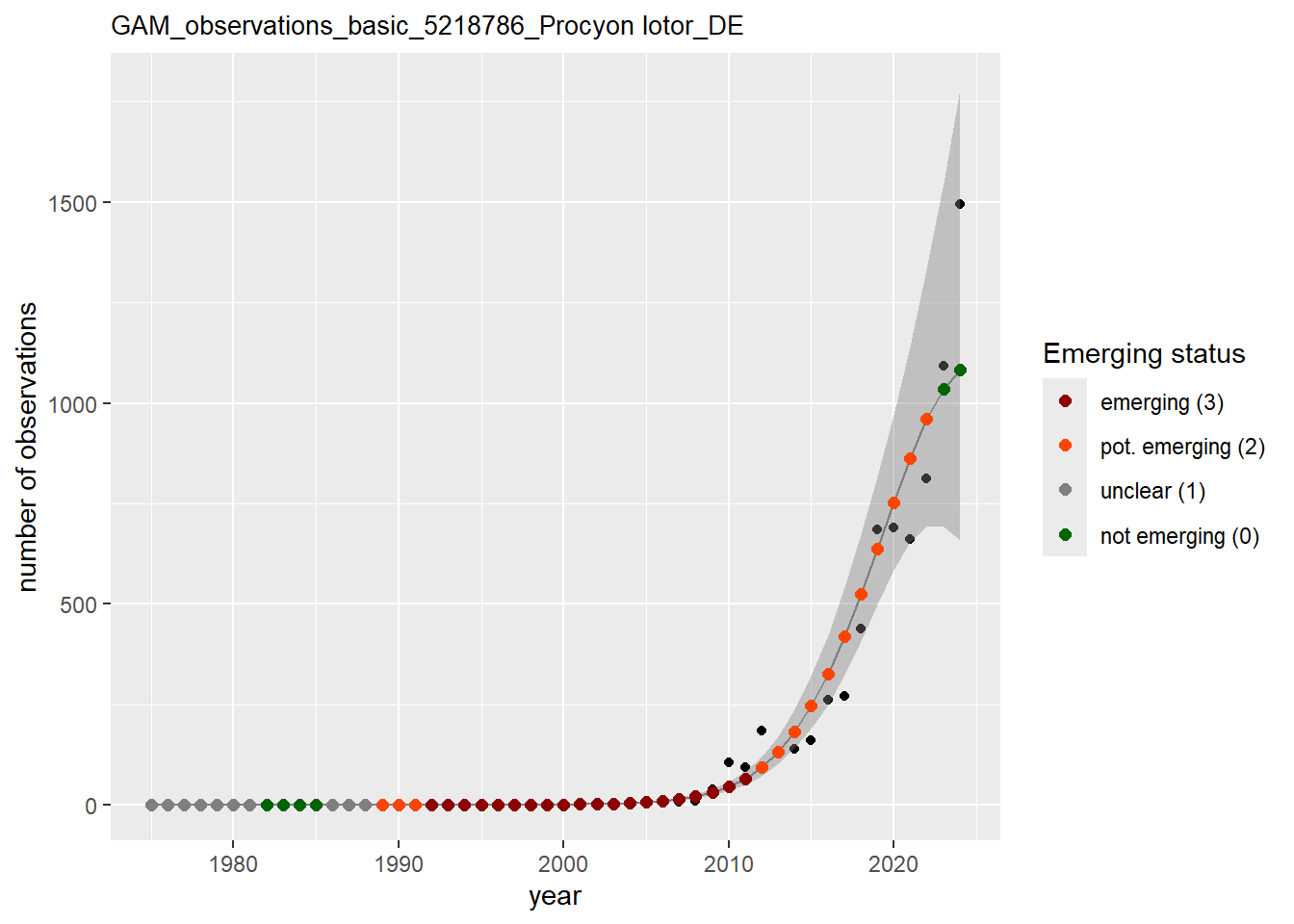
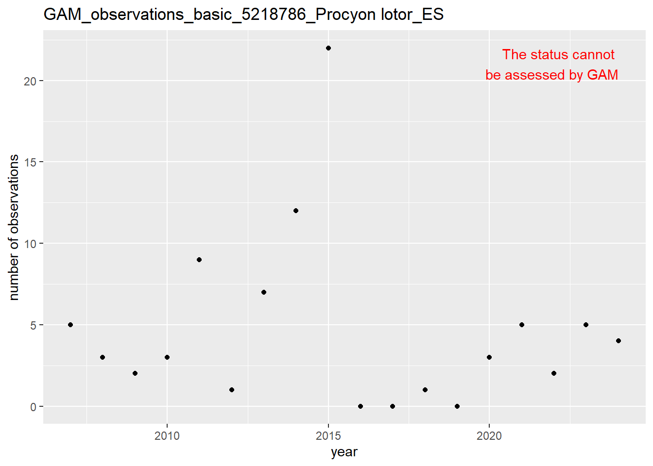
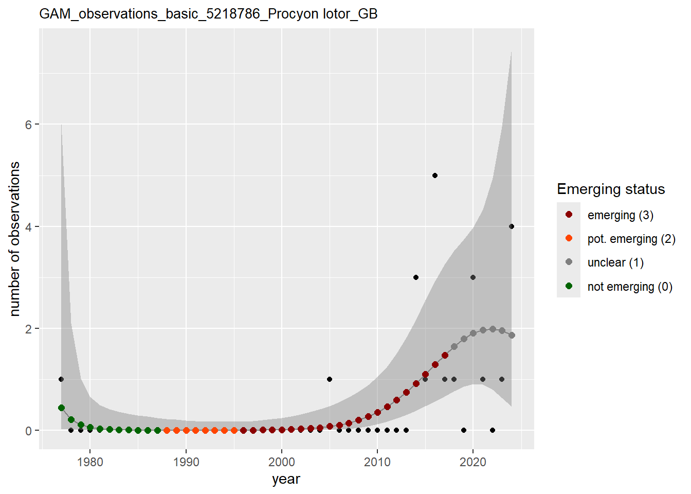
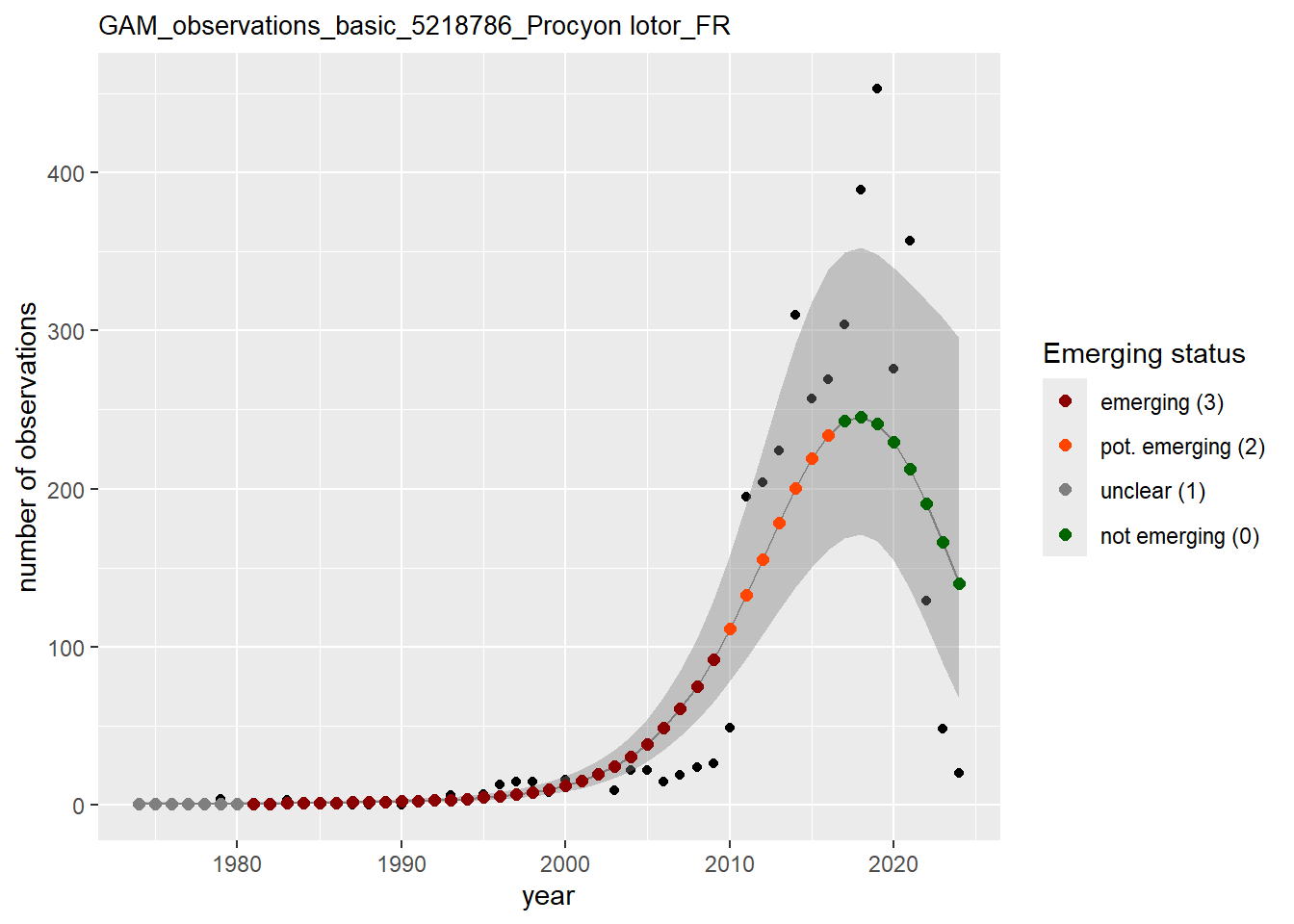
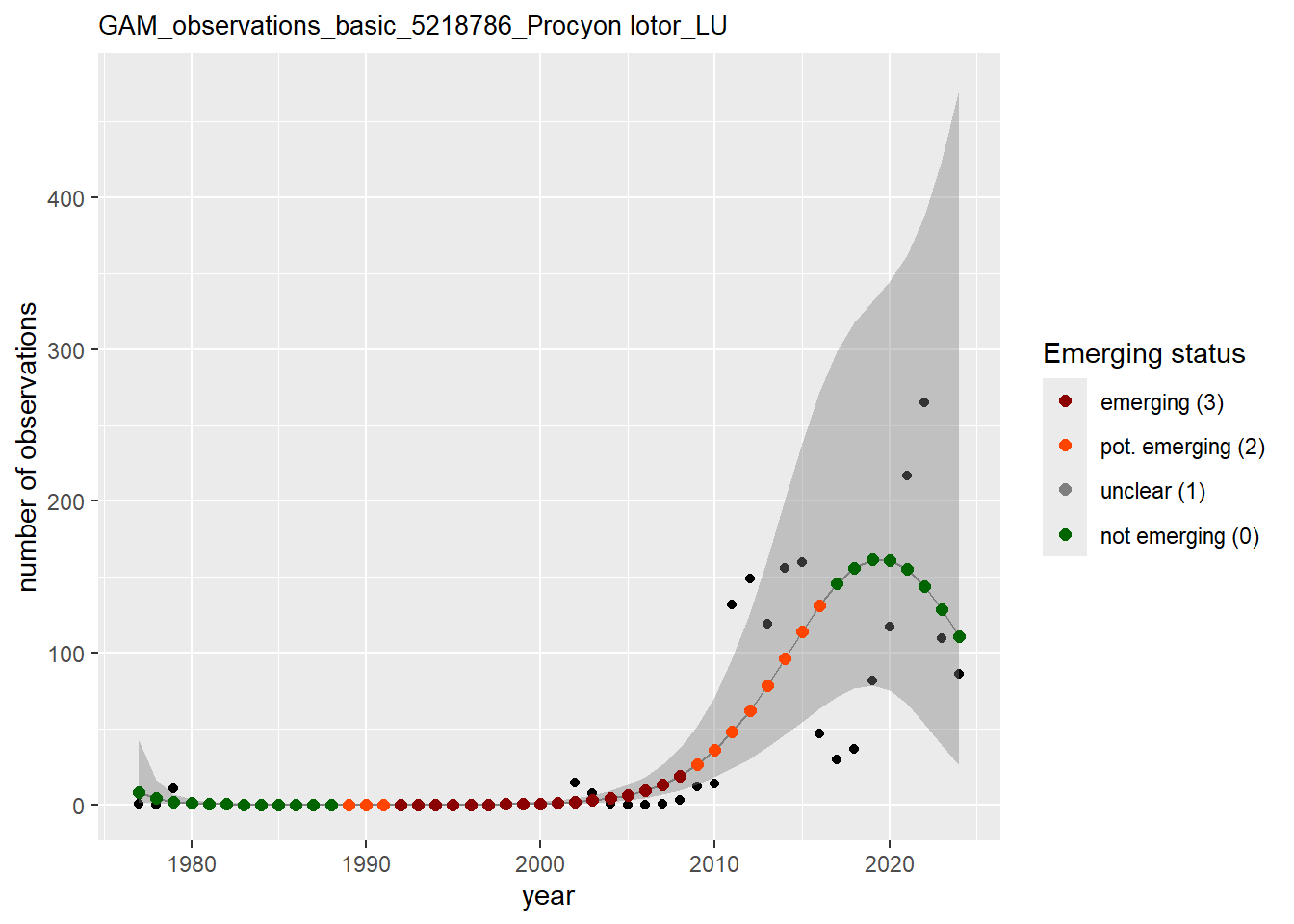
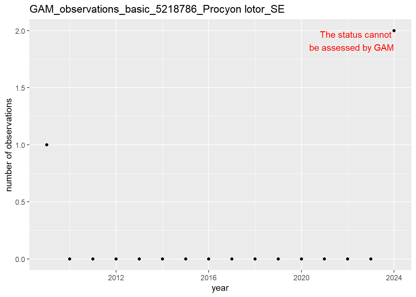
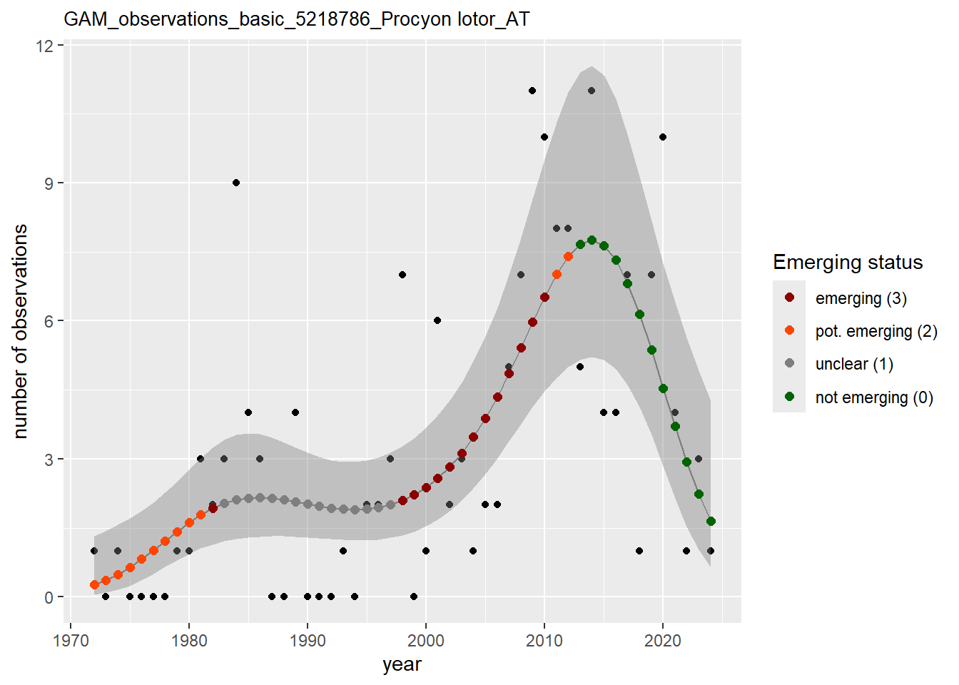
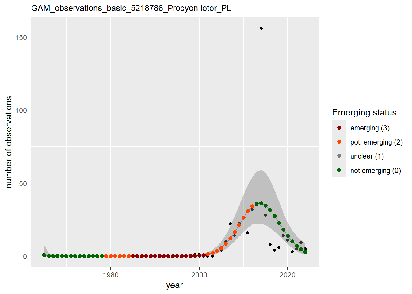
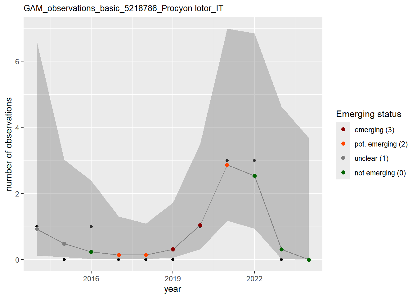
)We are now ready to apply a Generalized Additive Model (GAM) to assess the emerging status of raccoon.
eval_year <- 2024Let’s compact the time series:
compact_df_ts <- df_ts |>
    dplyr::group_by(specieskey, countrycode, year) |>
    dplyr::summarise(
      occs = sum(occurrences),
      ncells = sum(ispresent),
      .groups = "drop")
All plots will be saved in subdirectories of ./data/output/GAM_outputs:
dir_name_basic <- here::here("data", "output", "GAM_outputs")We also define the plot dimensions in pixels:
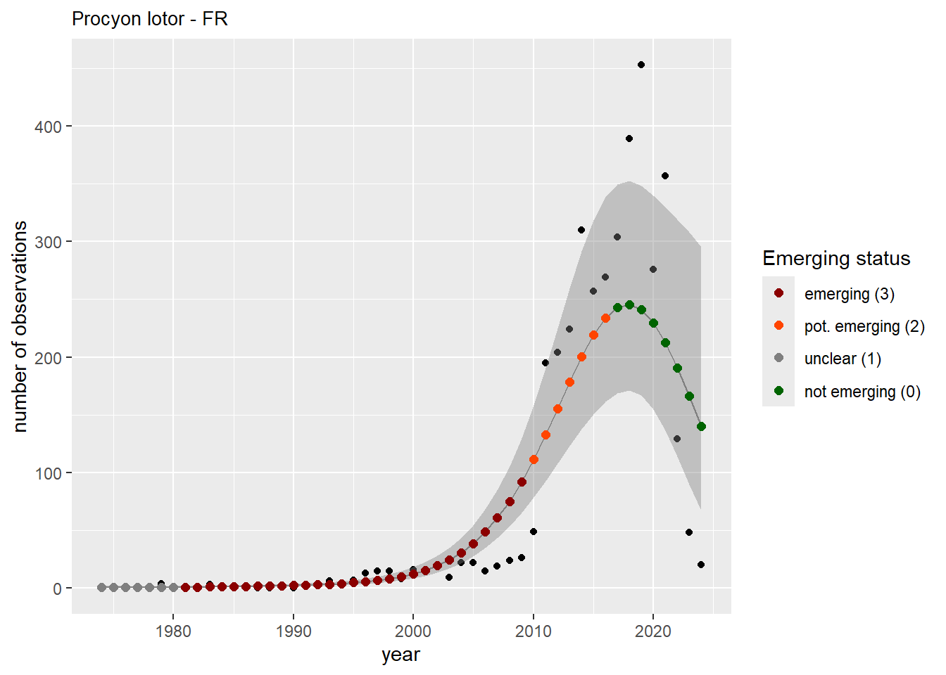
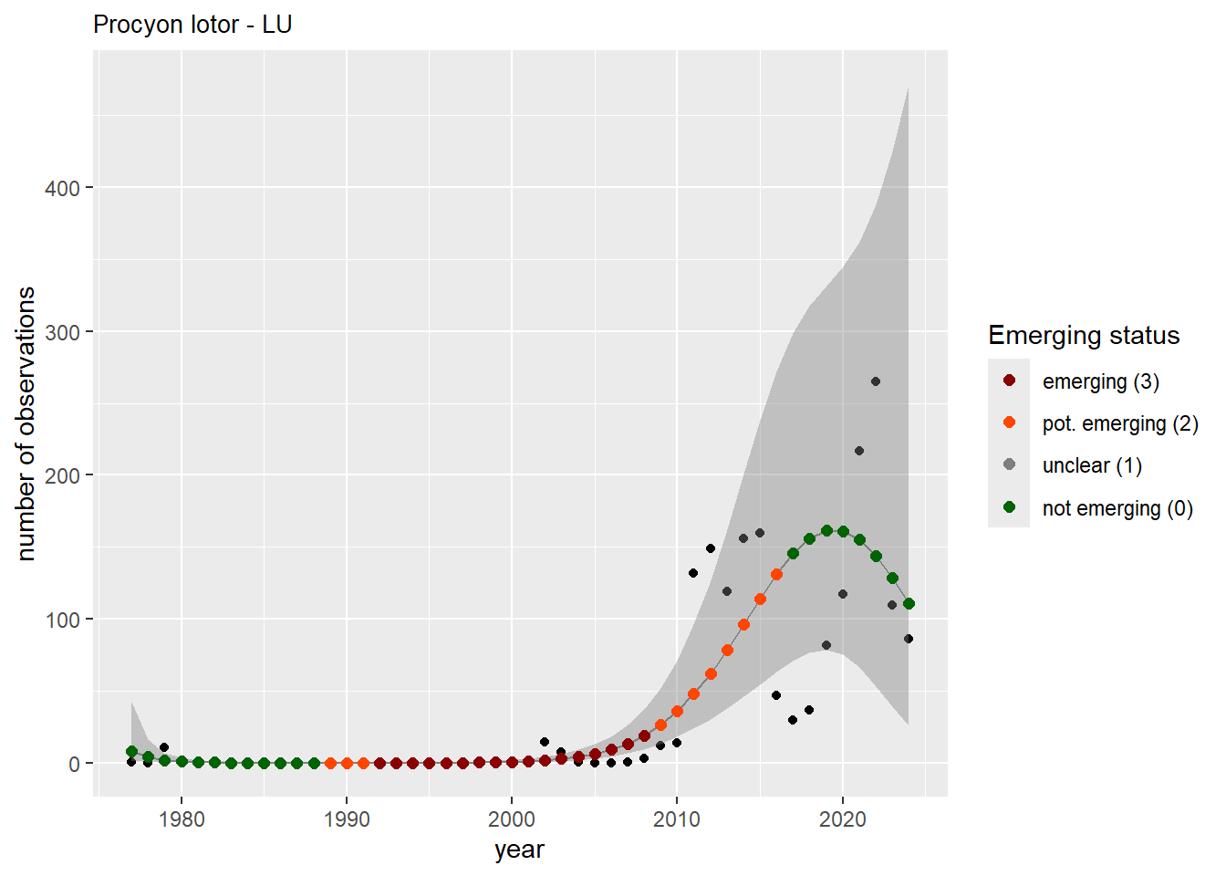
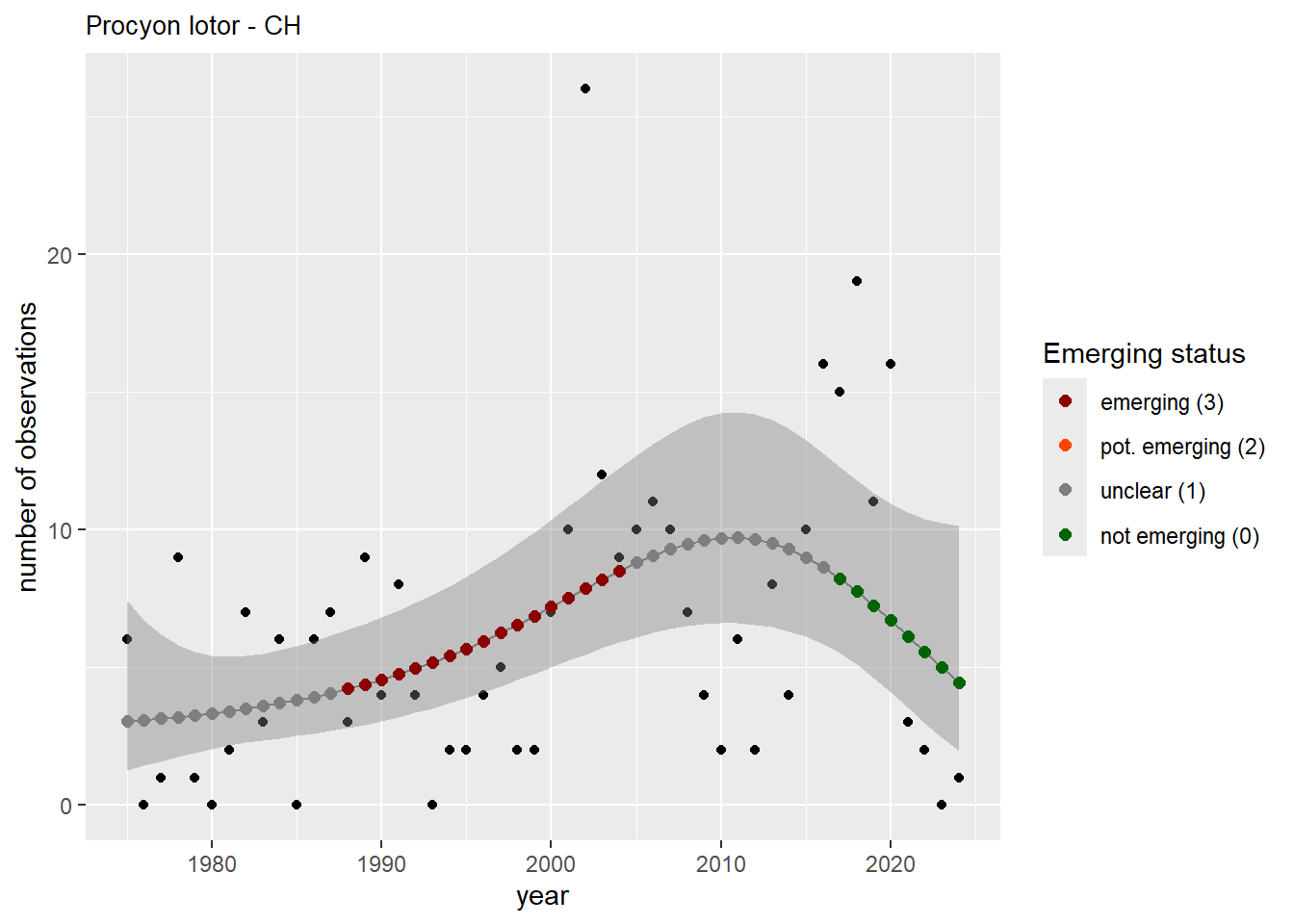
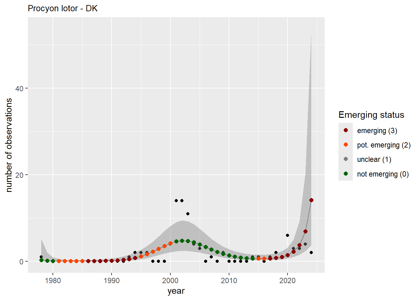
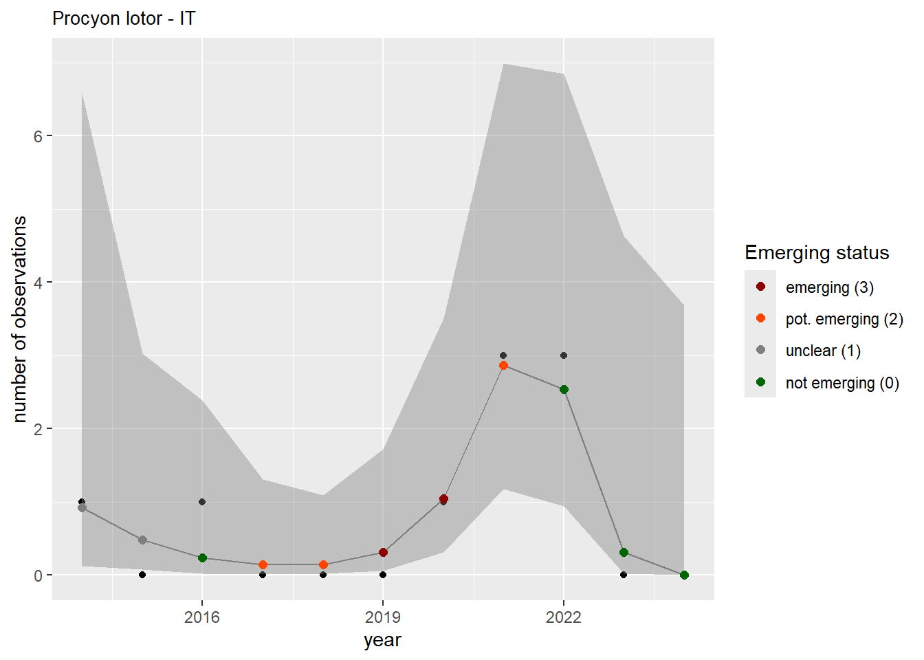
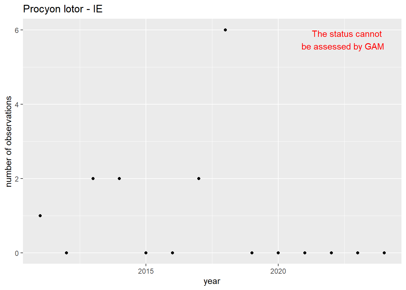
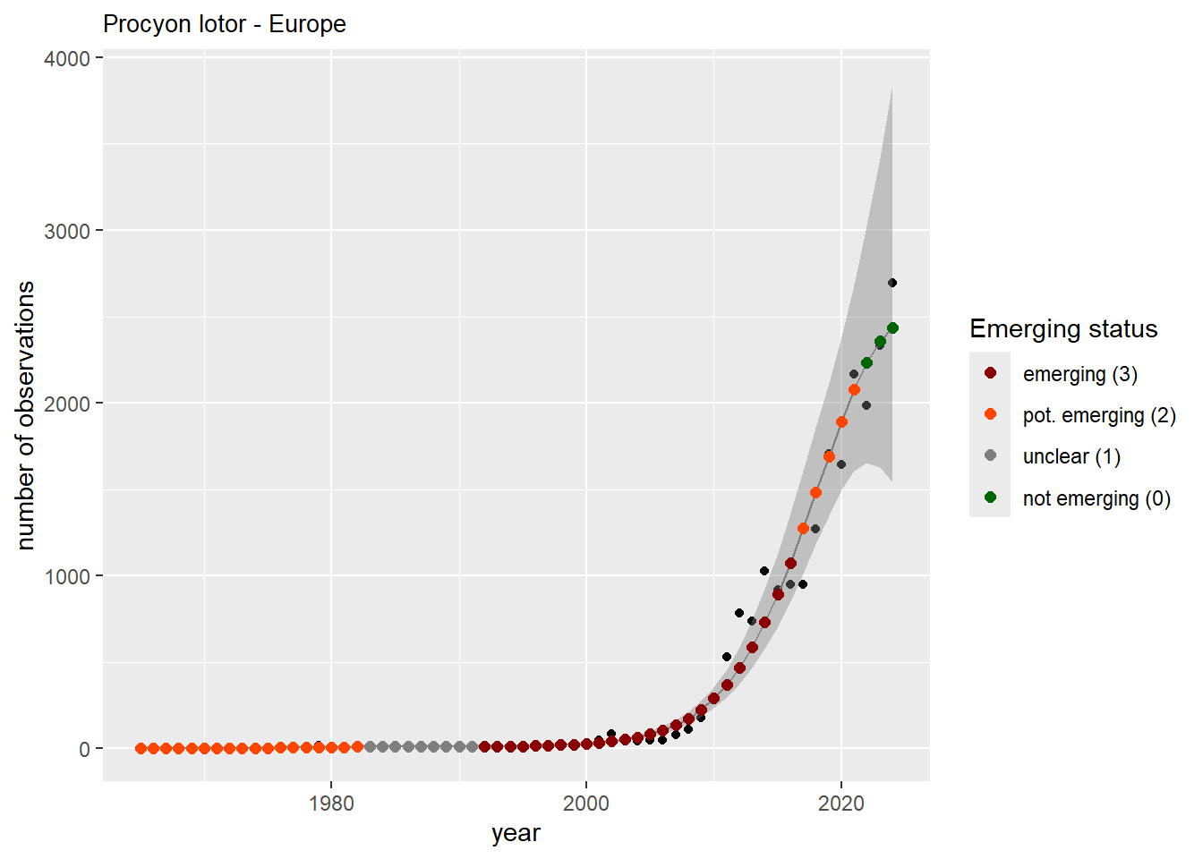
plot_dimensions <- list(width = 2800, height = 1500)We apply GAM for each country for the number of occurrences:
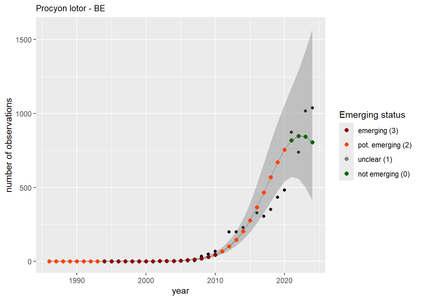
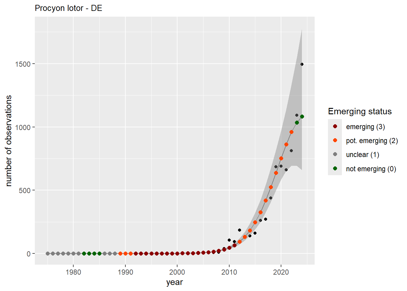
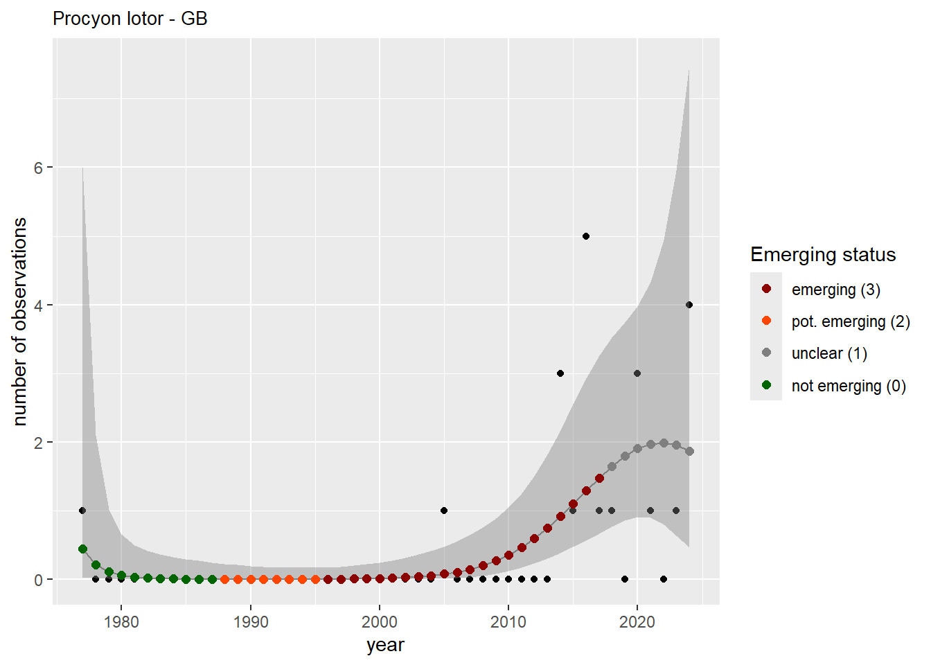
gam_occs <- purrr::map(
countrycode,
function(code) {
gam_occs_per_country <- purrr::map2(
species$specieskey, species$canonical_name,
function(t, n) {
df_key <- compact_df_ts |>
dplyr::filter(specieskey == t, countrycode == code)
trias::apply_gam(
df = df_key,
y_var = "occs",
taxonKey = "specieskey",
eval_years = 2024,
type_indicator = "observations",
taxon_key = t,
name = n,
df_title = code,
dir_name = paste0(dir_name_basic, "/long_titles"),
y_label = "number of observations",
saveplot = TRUE,
width = plot_dimensions$width,
height = plot_dimensions$height
)
})
names(gam_occs_per_country) <- species$canonical_name
gam_occs_per_country
}
)
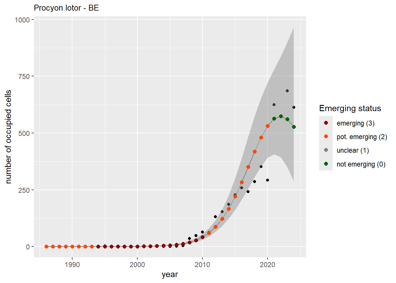
names(gam_occs) <- countrycodeAnd the number of occupied cells, or measured occupancy:
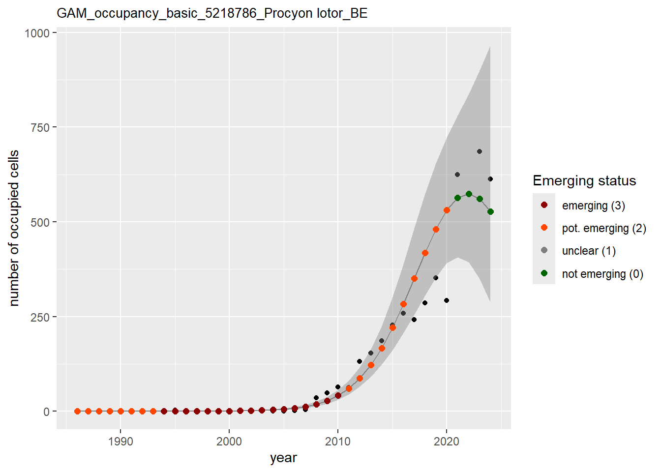
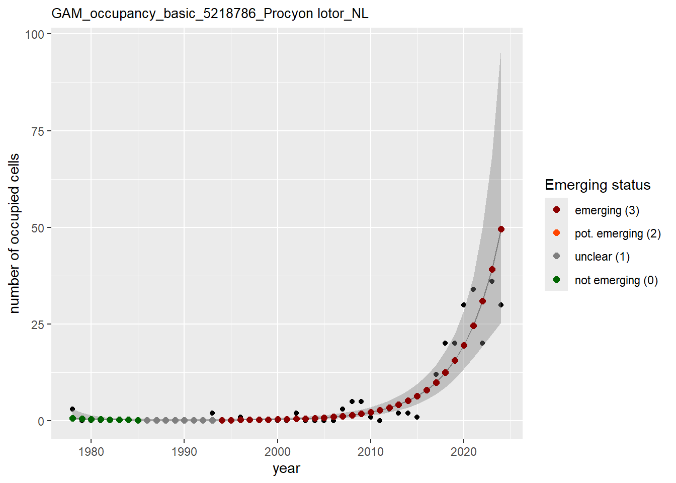
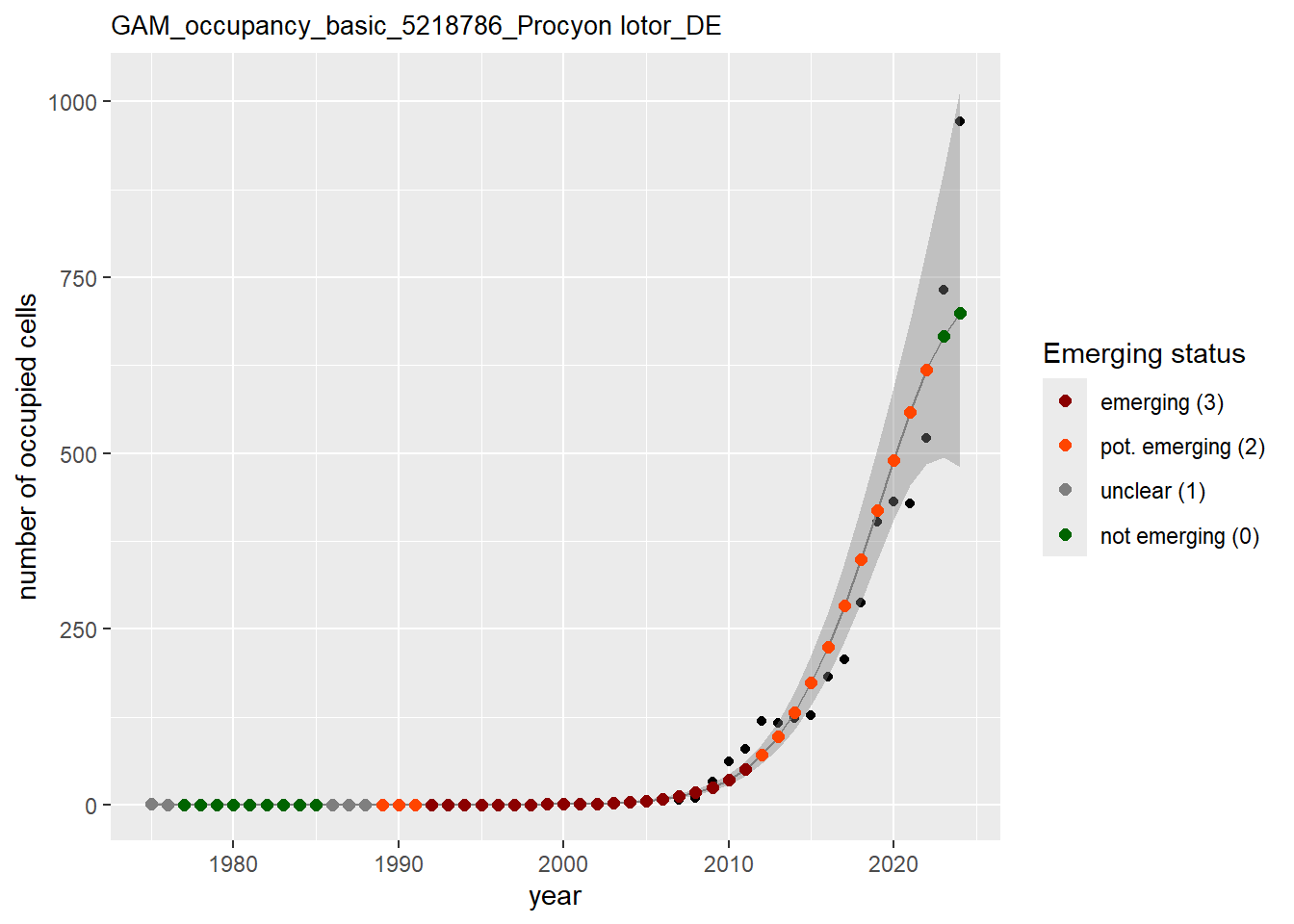
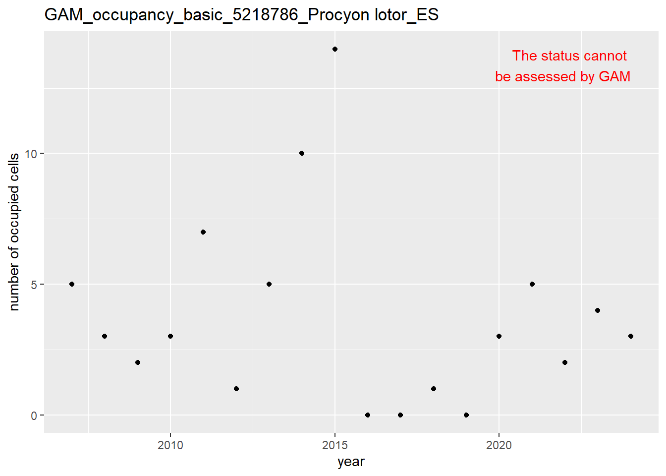
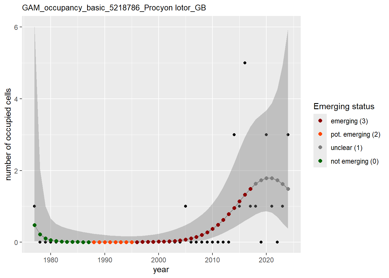
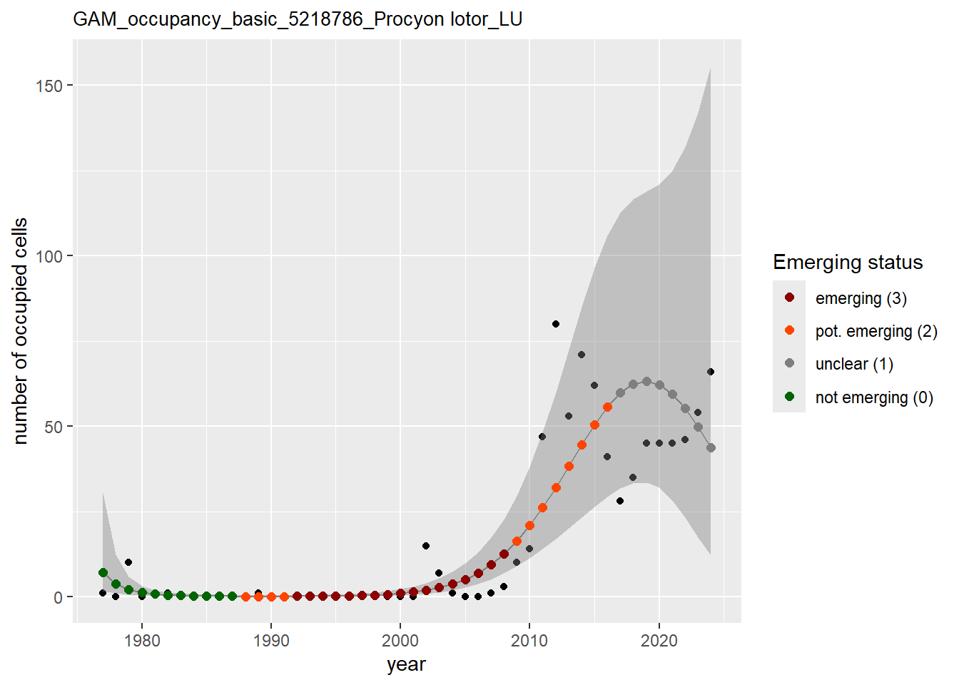
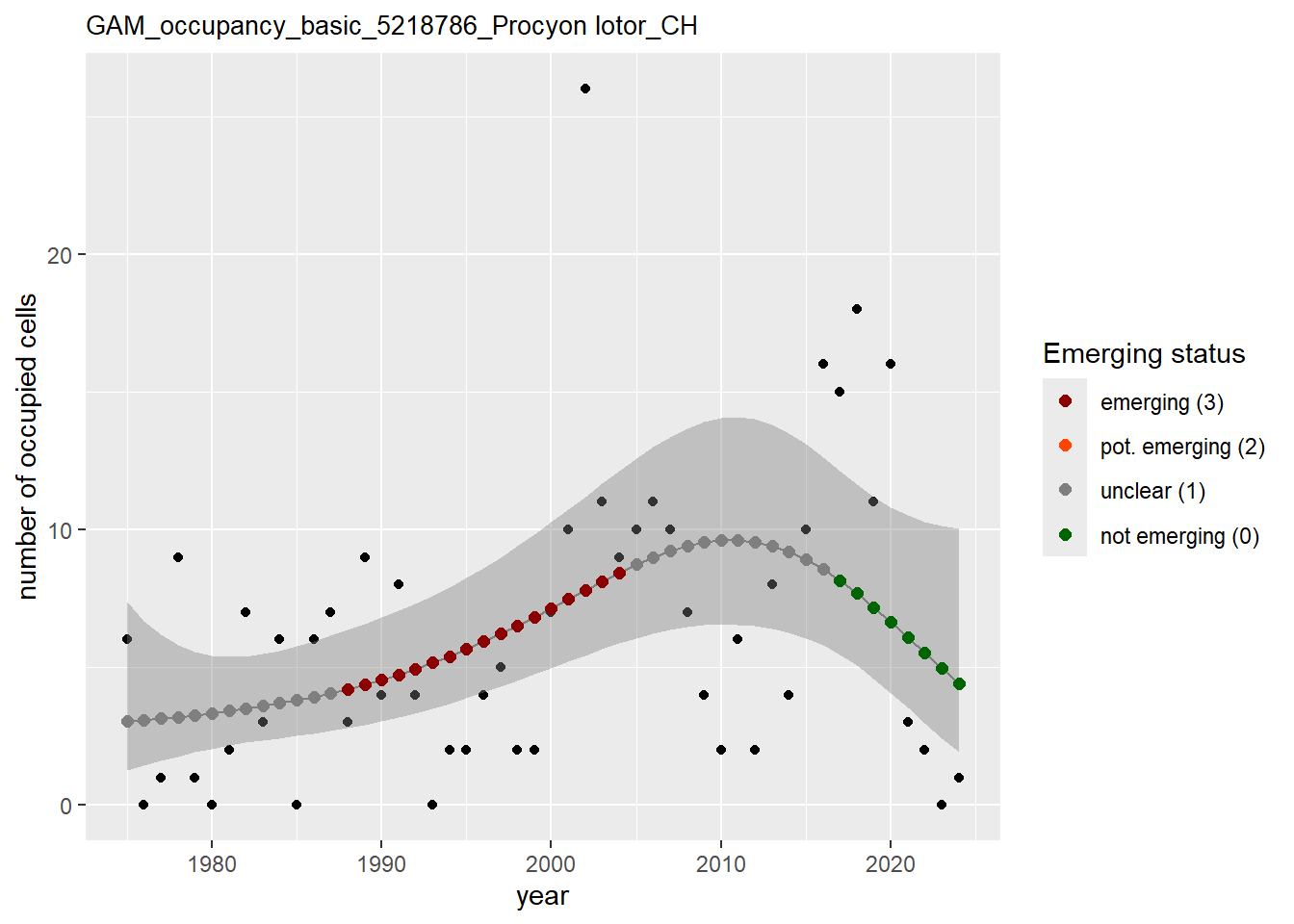
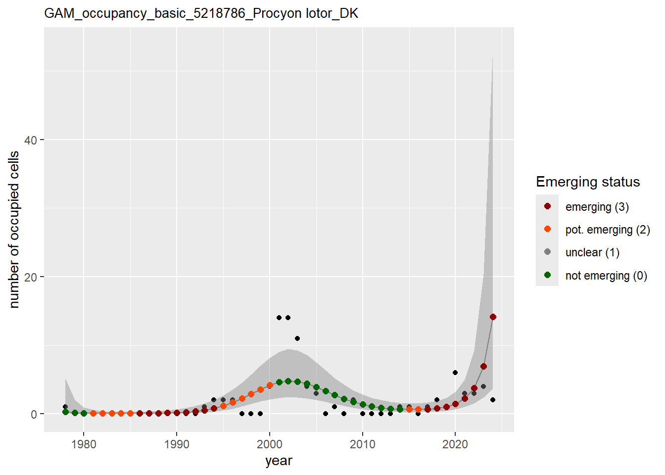
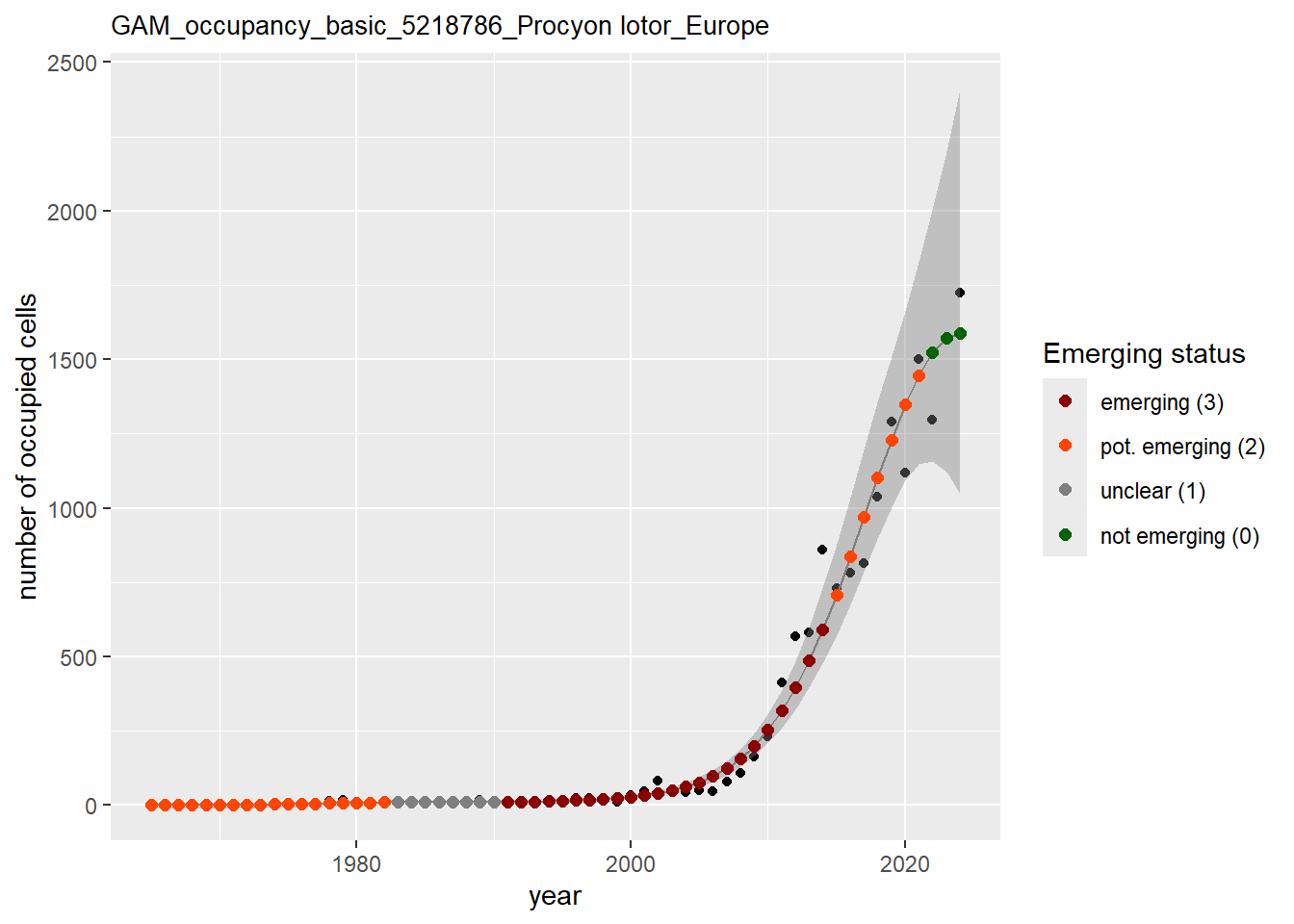
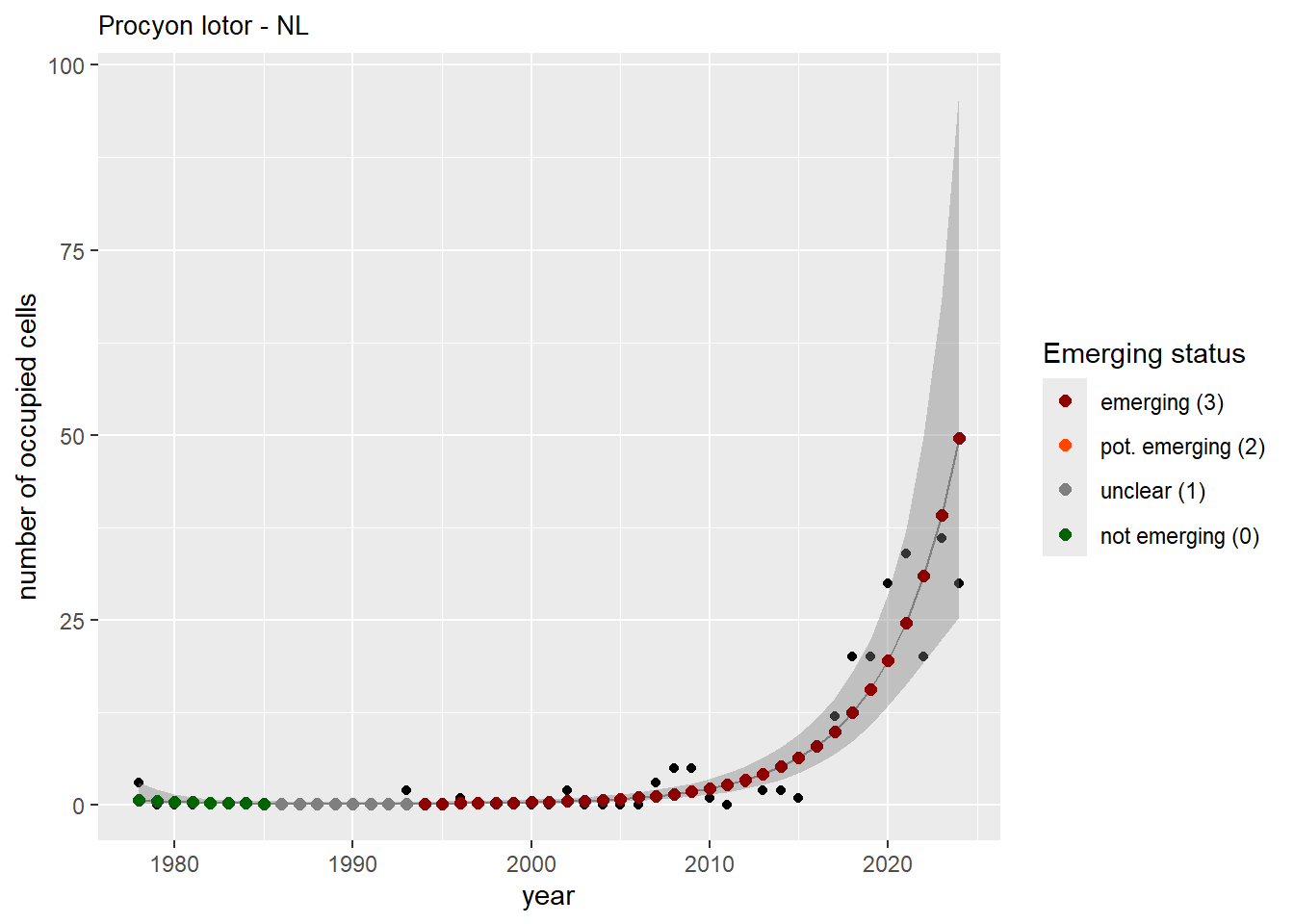
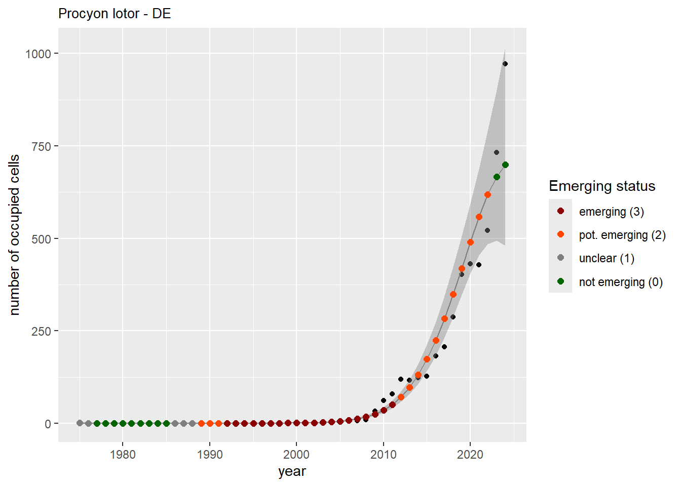
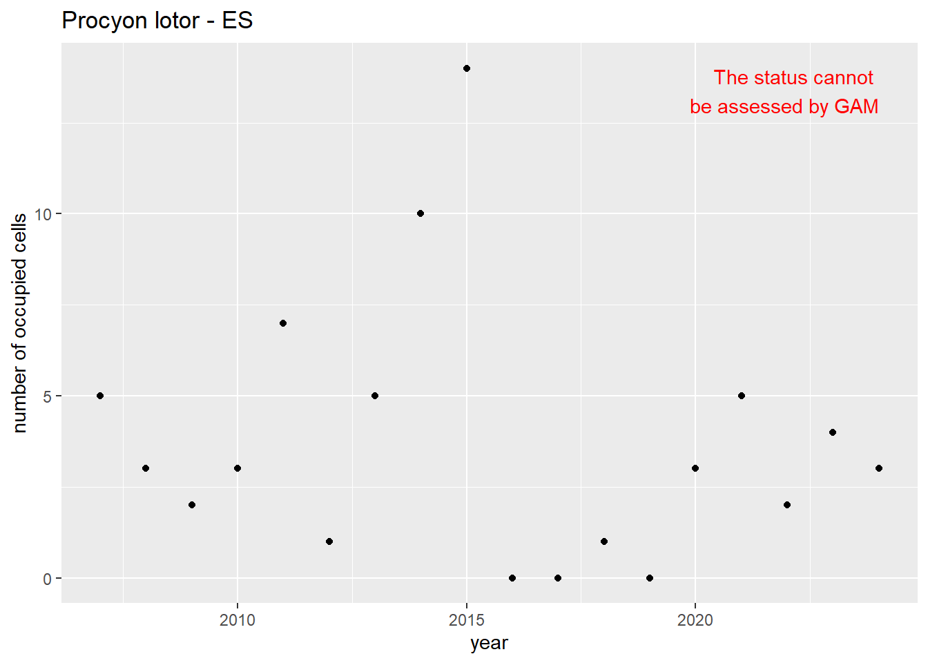
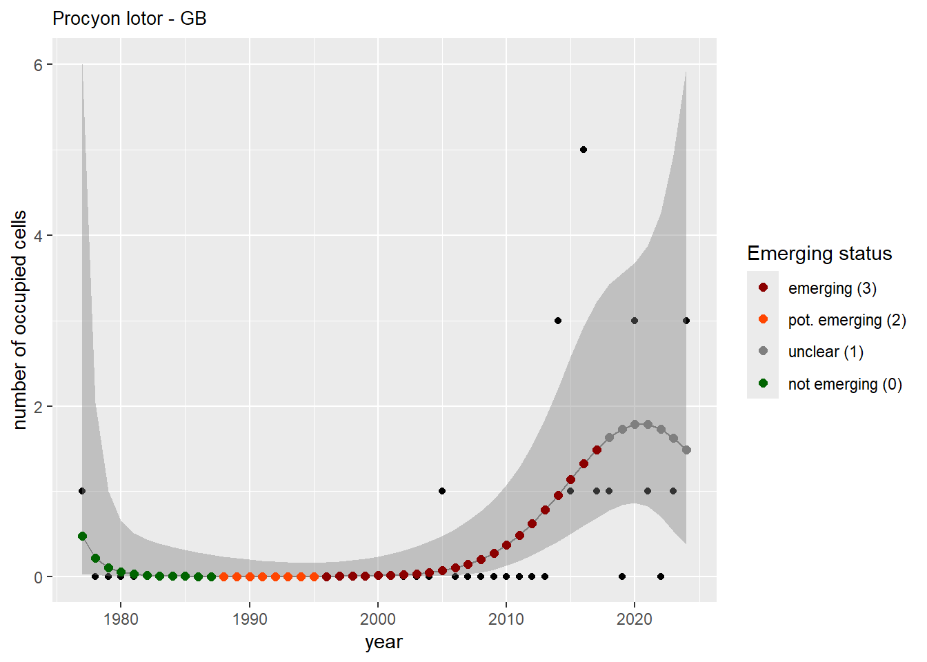
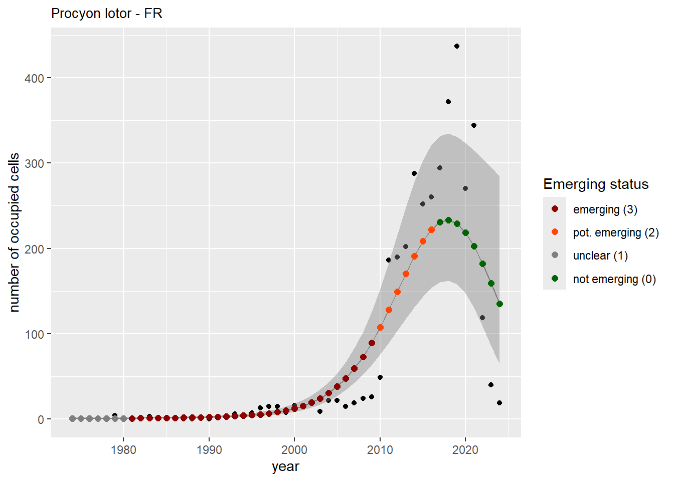
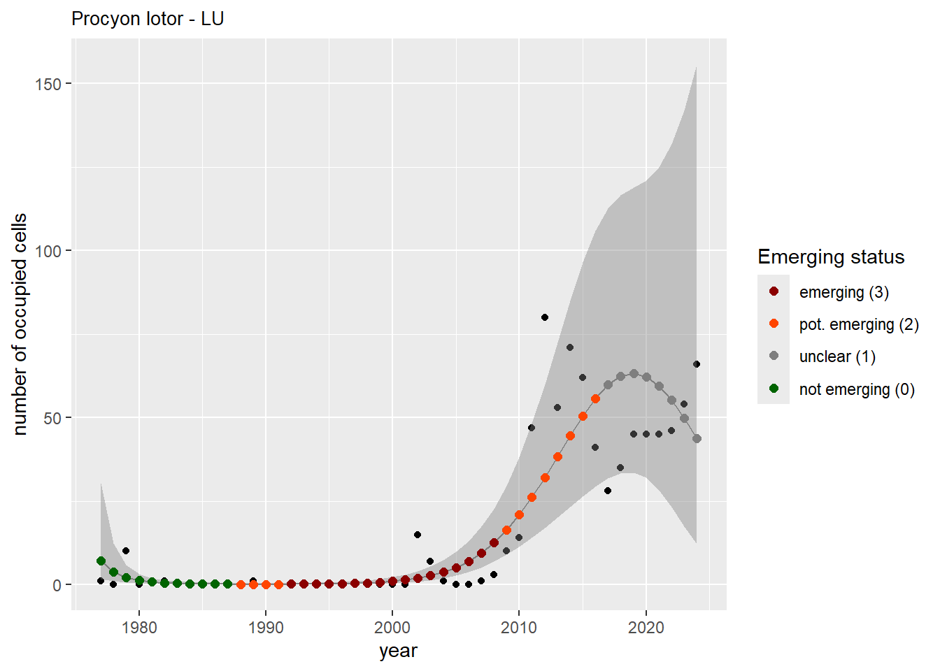
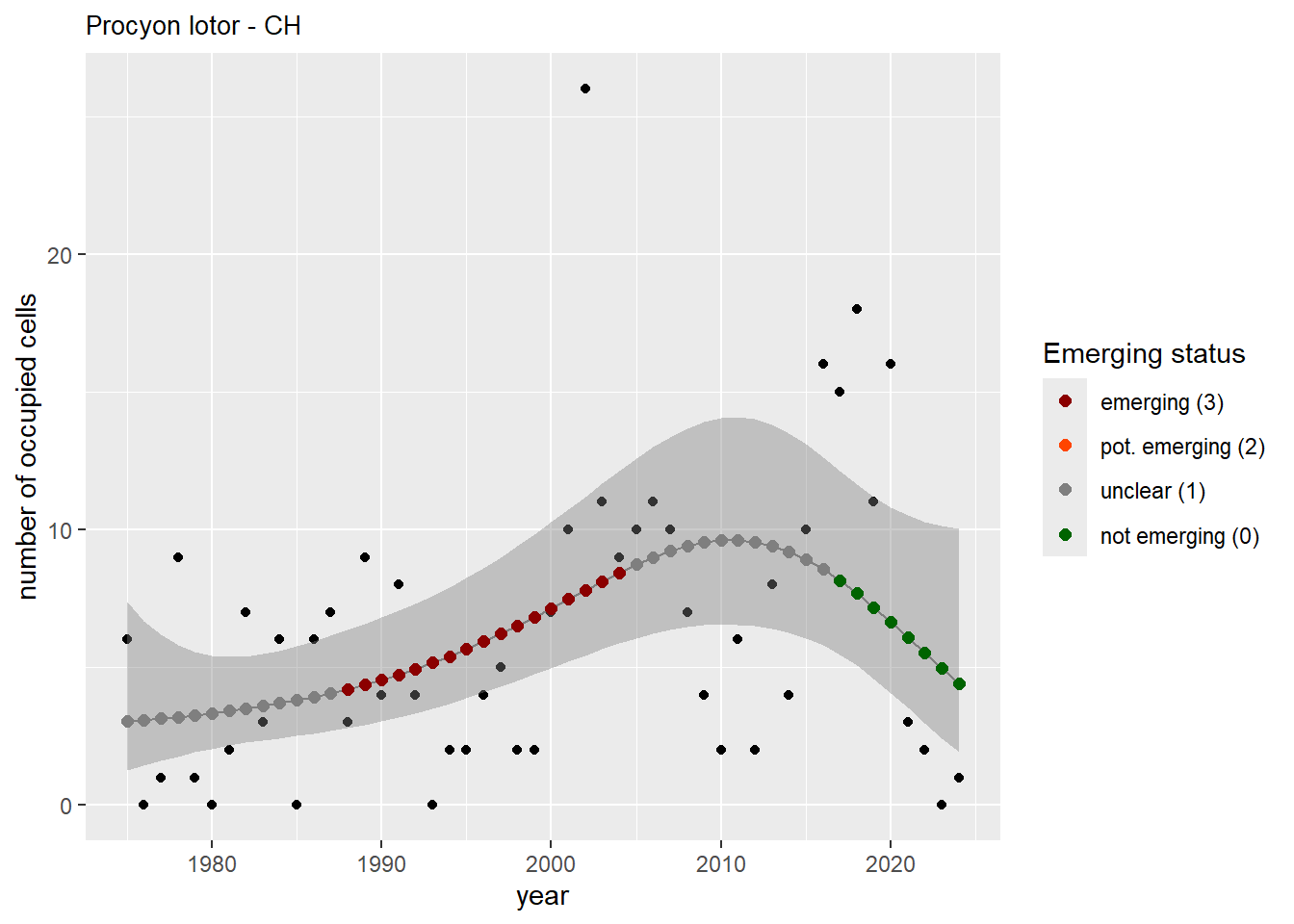
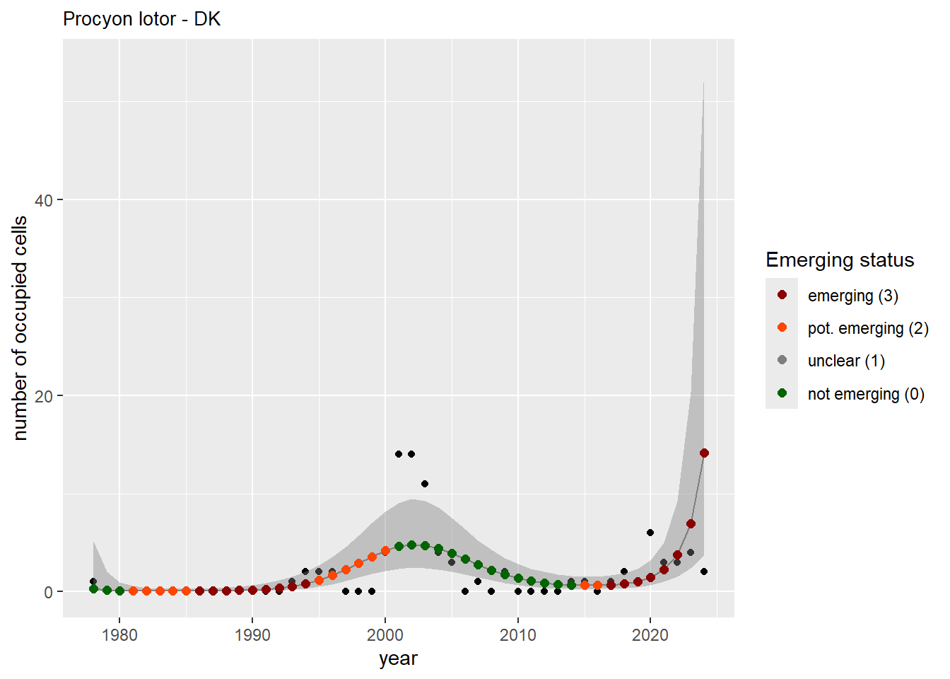
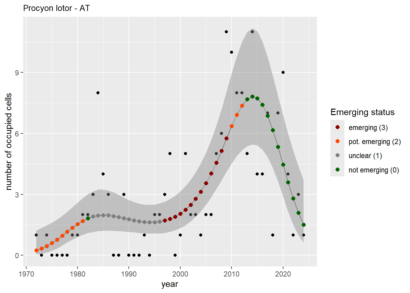
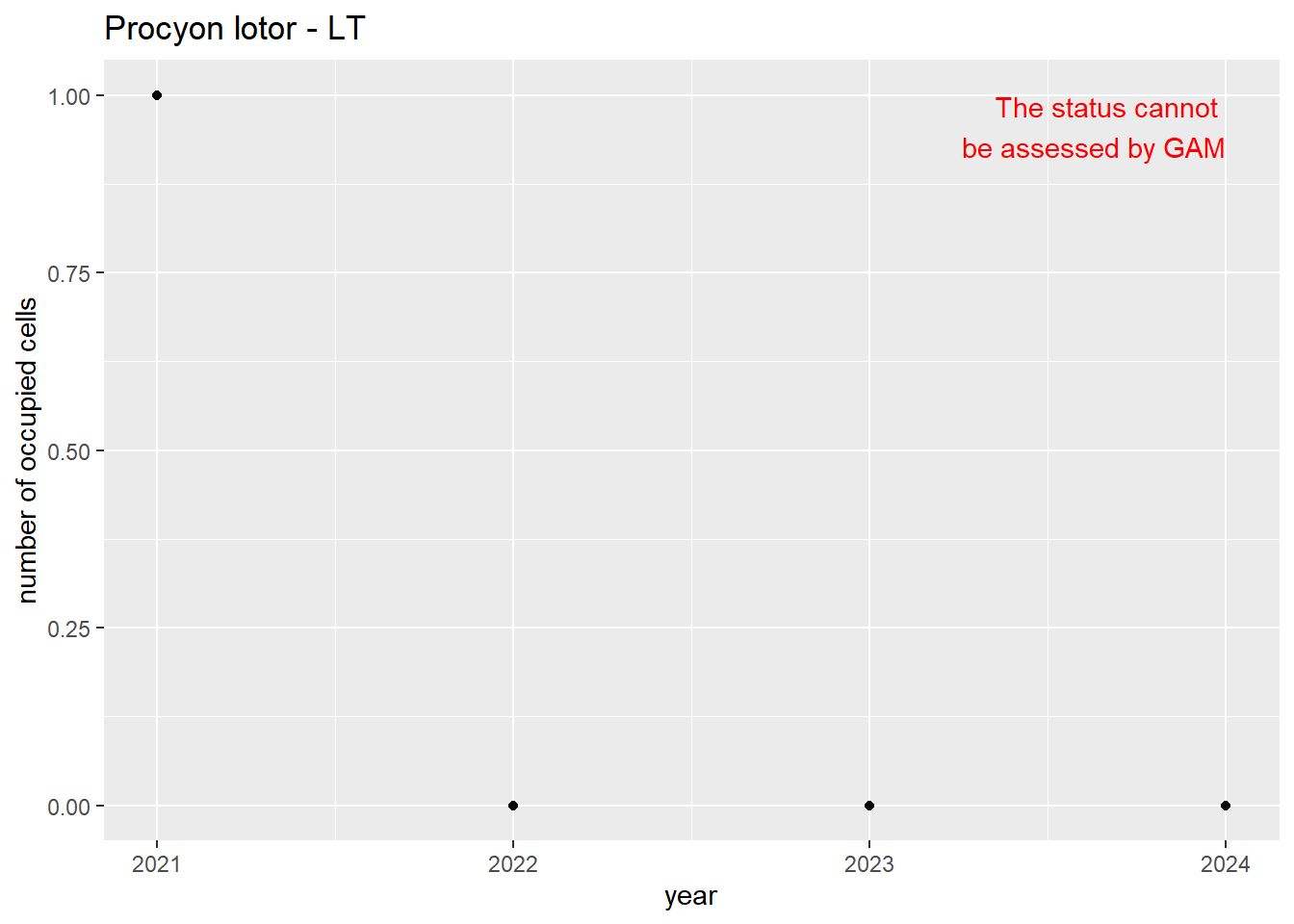
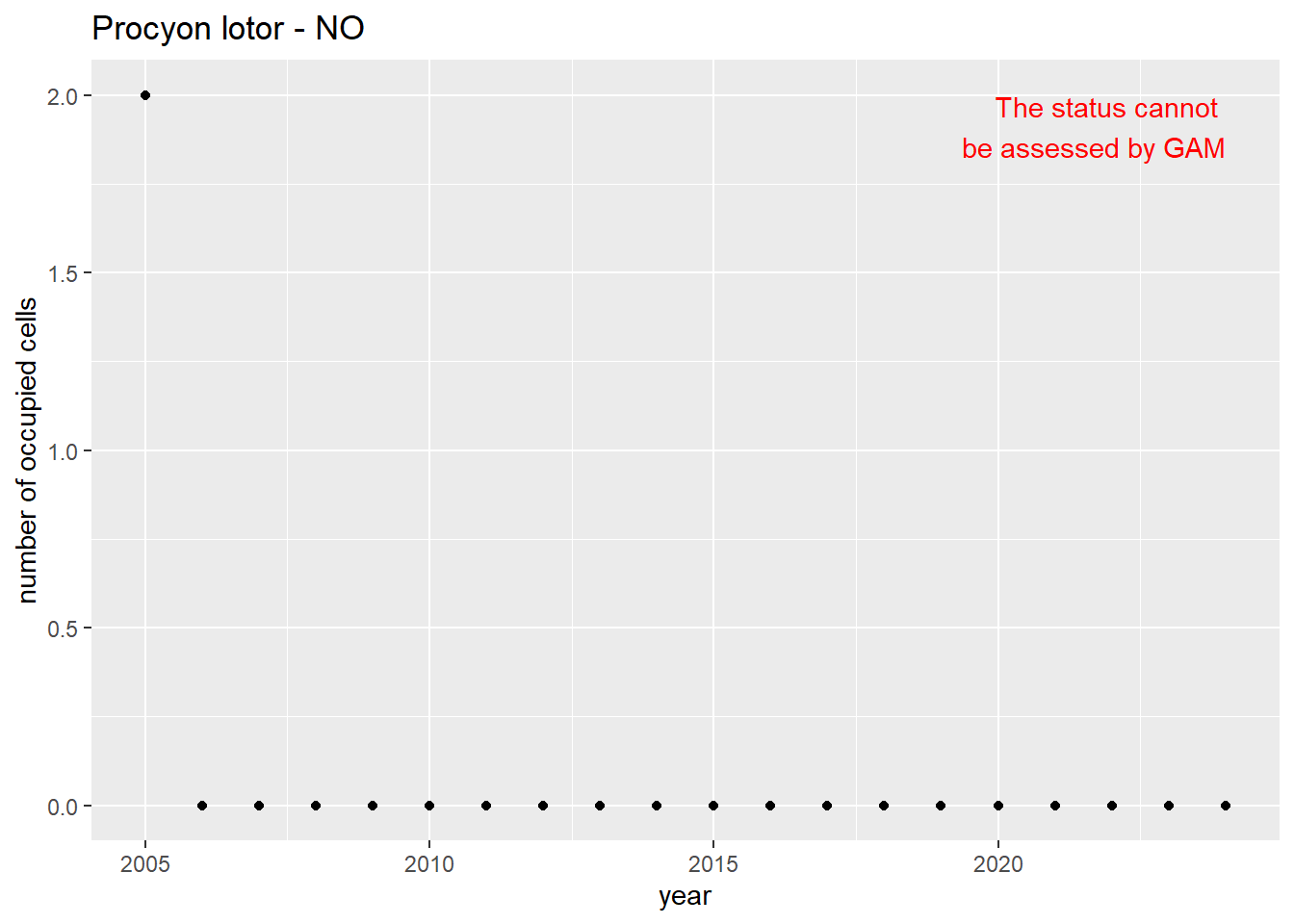
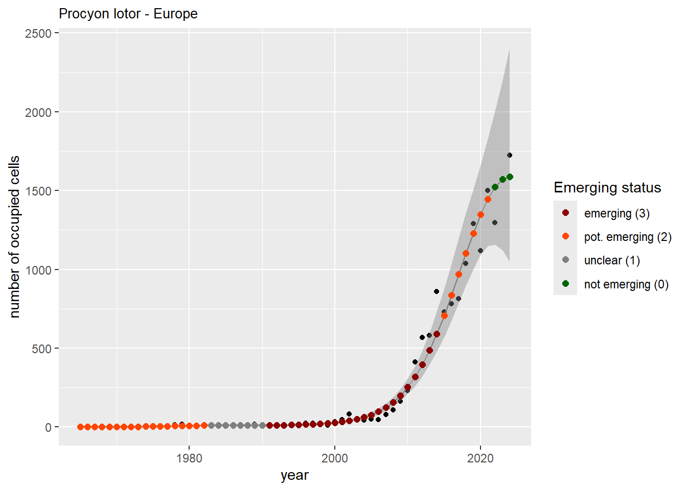
gam_ncells <- purrr::map(
countrycode,
function(code) {
gam_ncells_per_country <- purrr::map2(
species$specieskey, species$canonical_name,
function(t, n) {
df_key <- compact_df_ts |>
dplyr::filter(specieskey == t, countrycode == code)
trias::apply_gam(
df = df_key,
y_var = "ncells",
taxonKey = "specieskey",
eval_years = 2024,
type_indicator = "occupancy",
taxon_key = t,
name = n,
df_title = code,
dir_name = paste0(dir_name_basic, "/long_titles"),
y_label = "number of occupied cells",
saveplot = TRUE,
width = plot_dimensions$width,
height = plot_dimensions$height
)
})
names(gam_ncells_per_country) <- species$canonical_name
gam_ncells_per_country
}
)
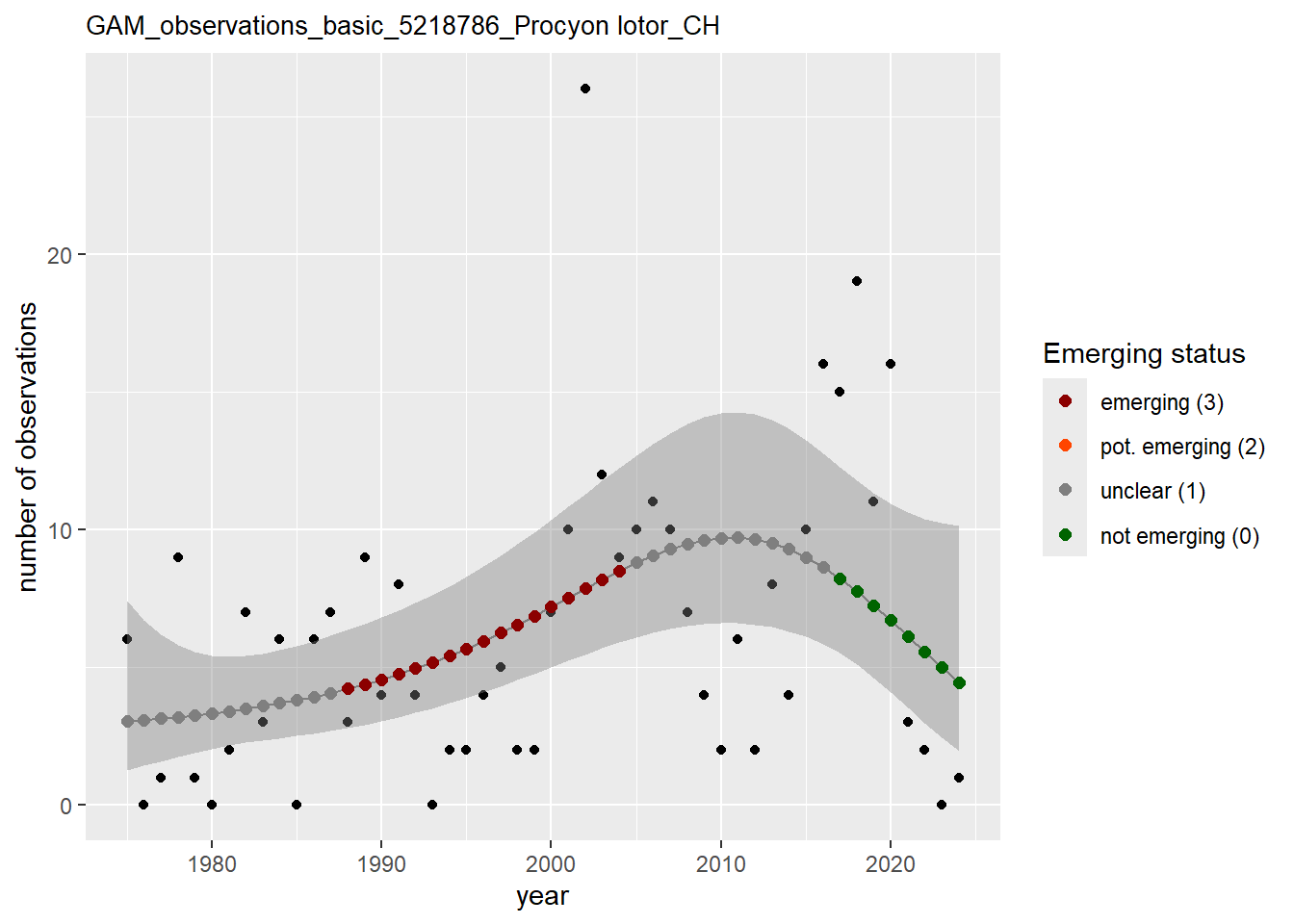
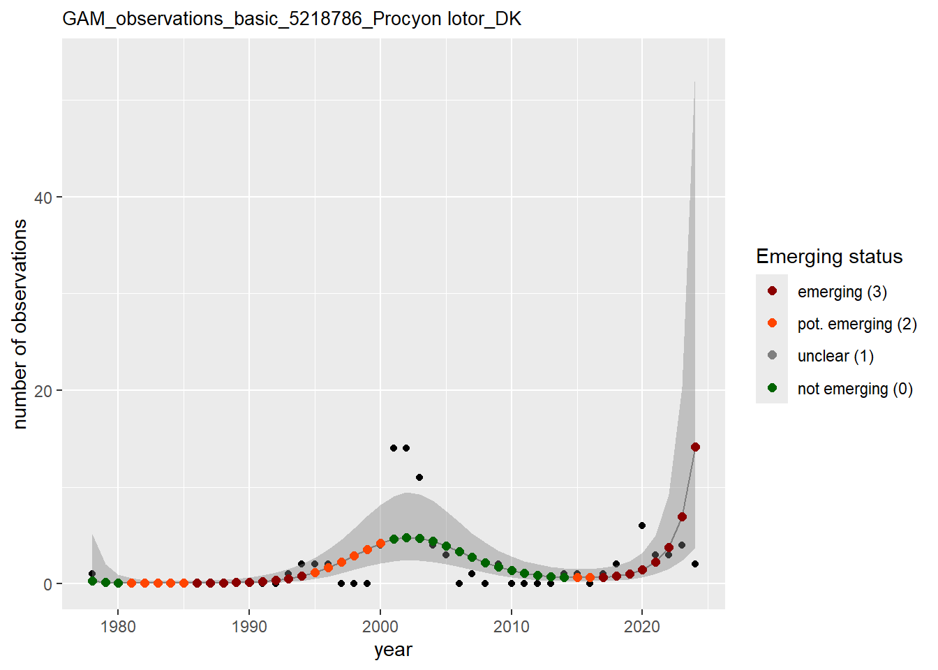
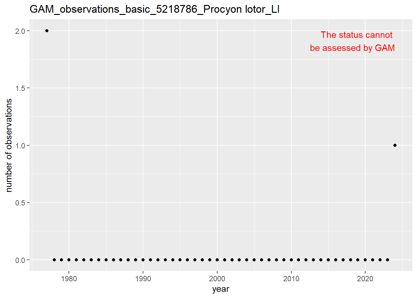
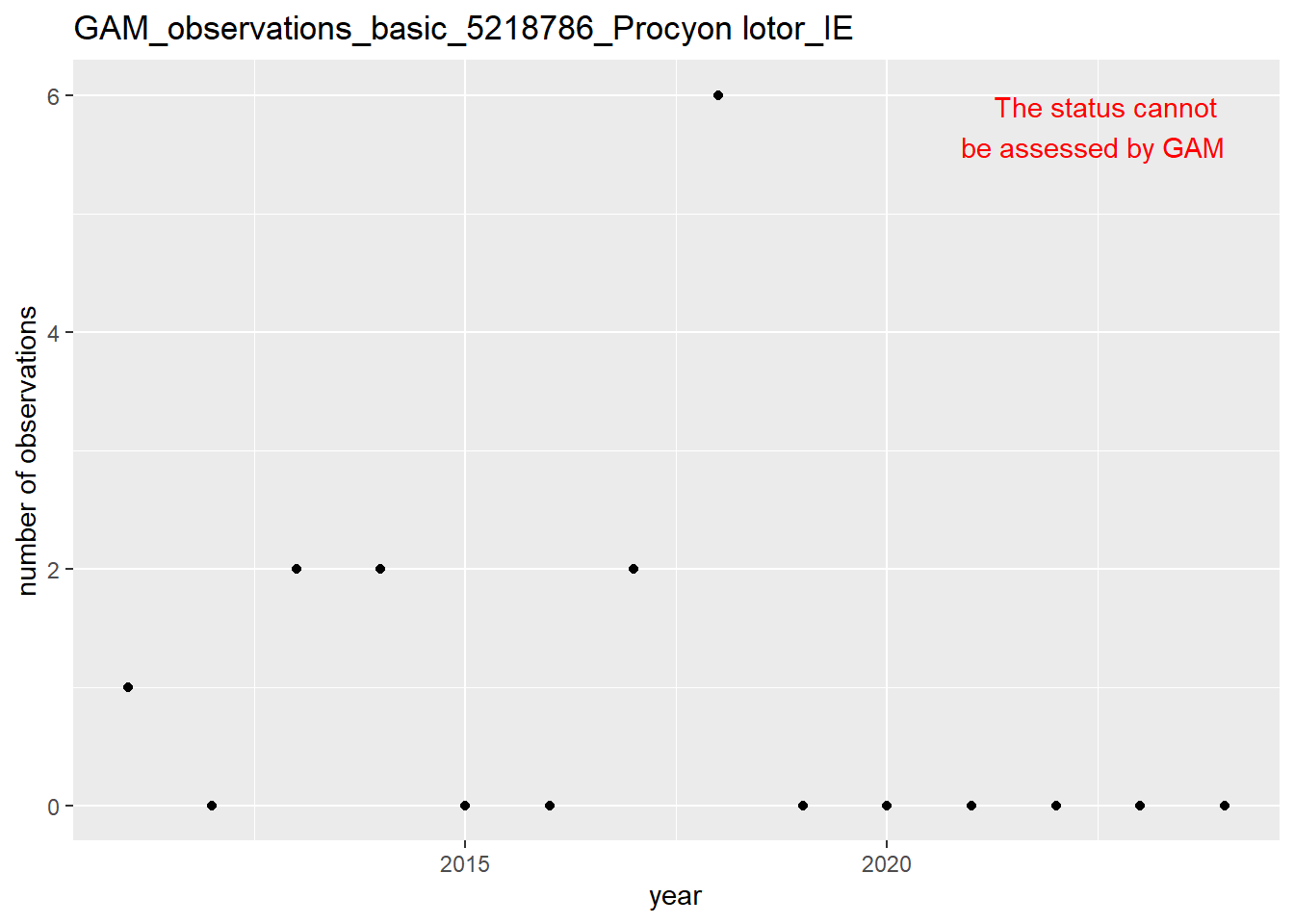
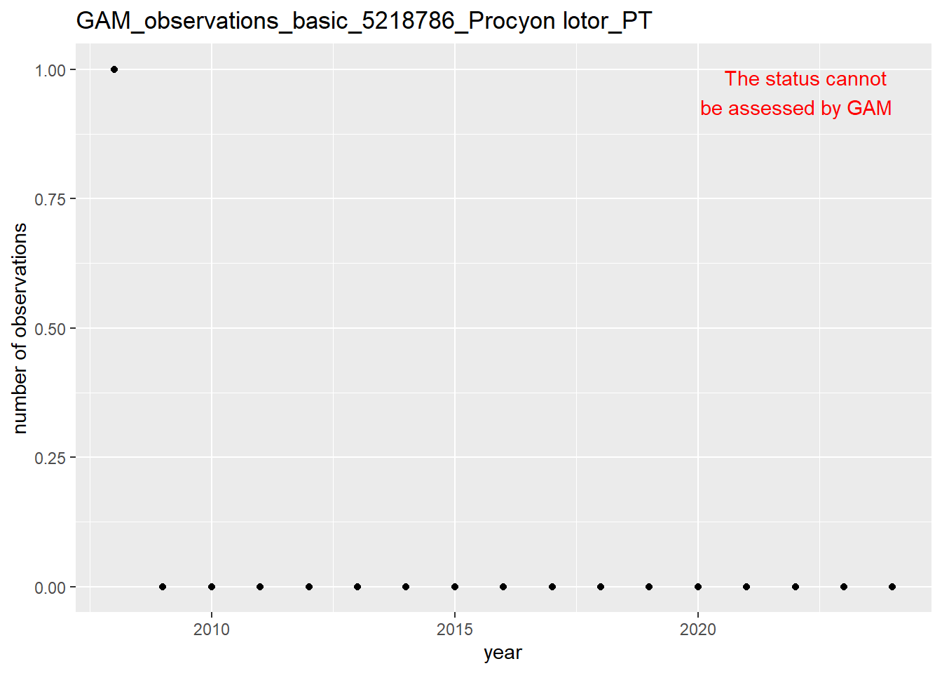
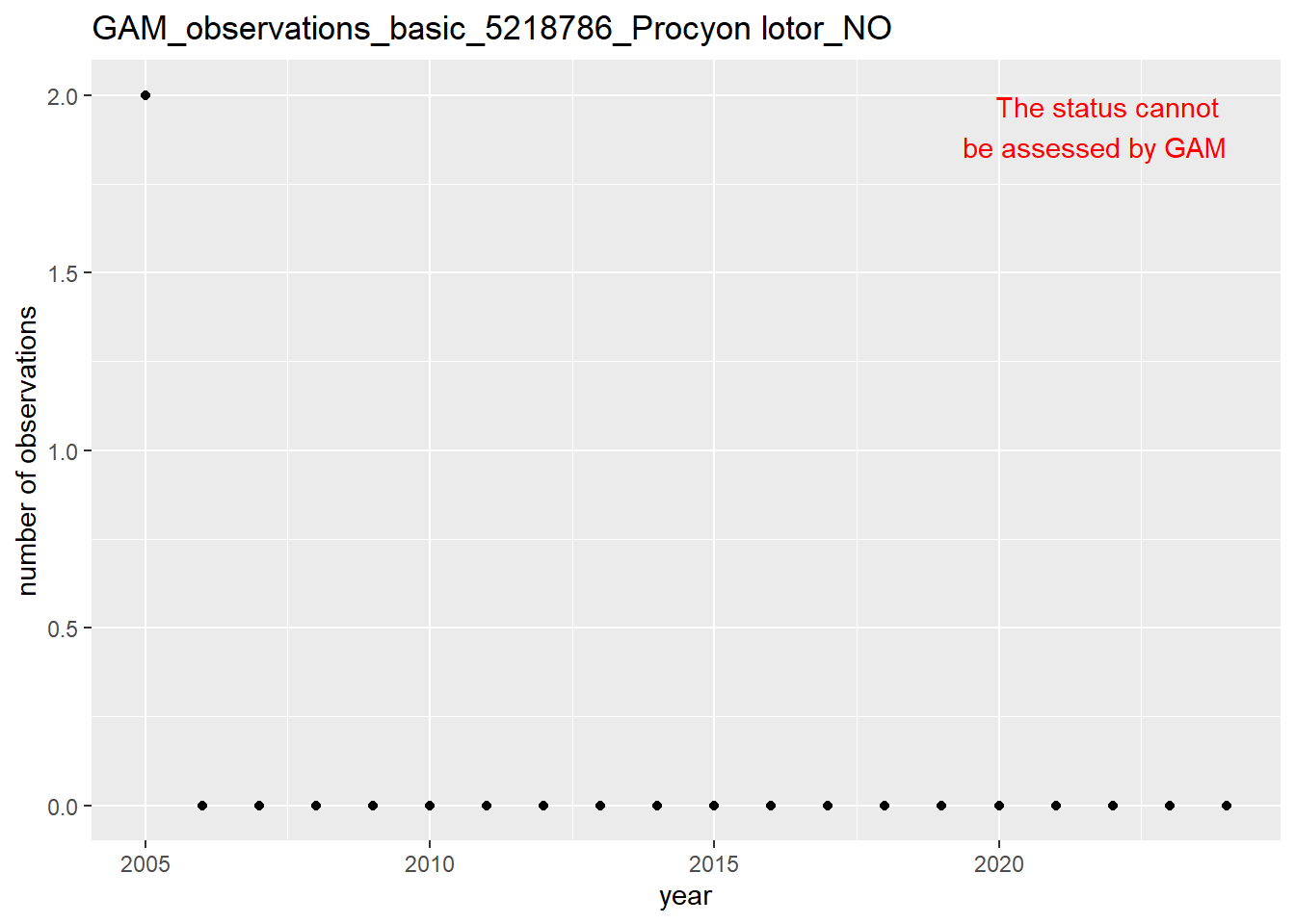
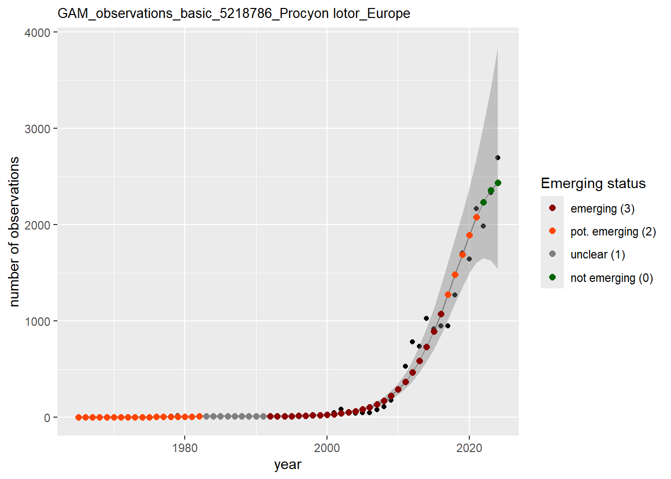
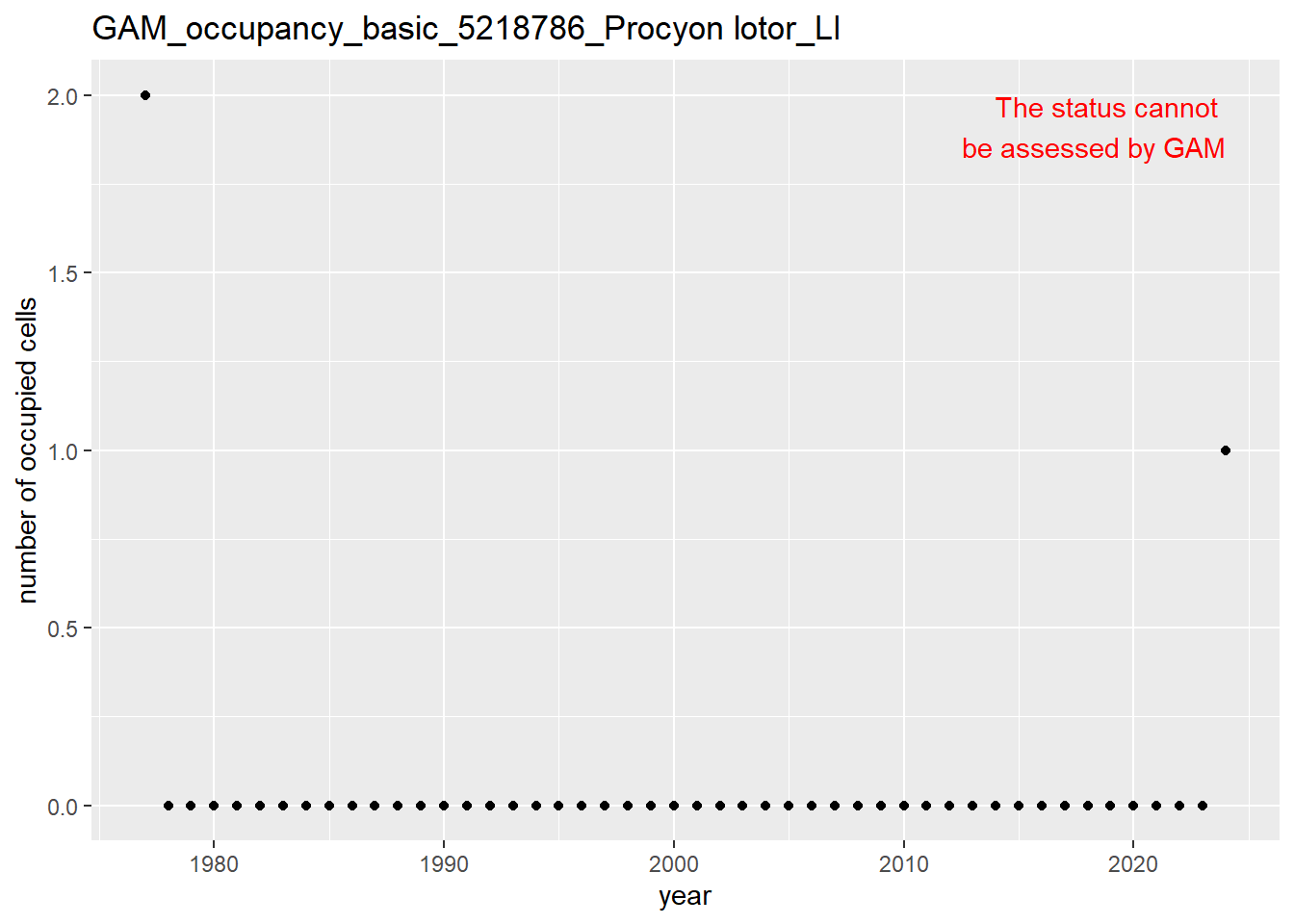
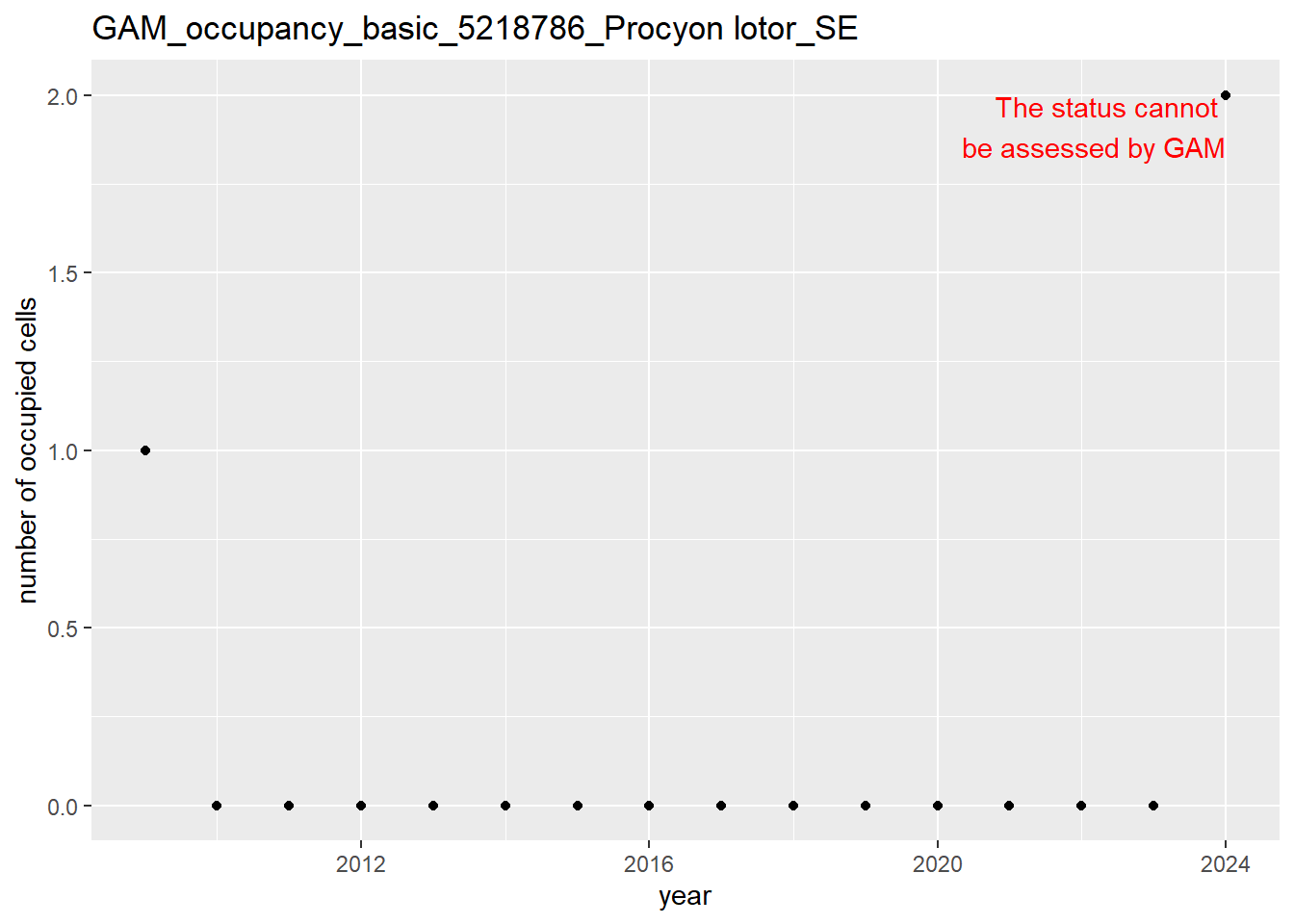
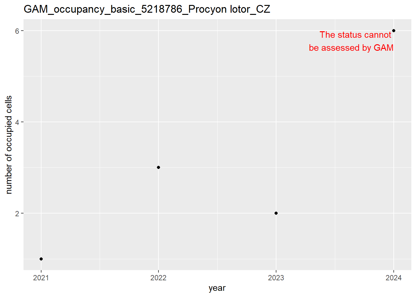
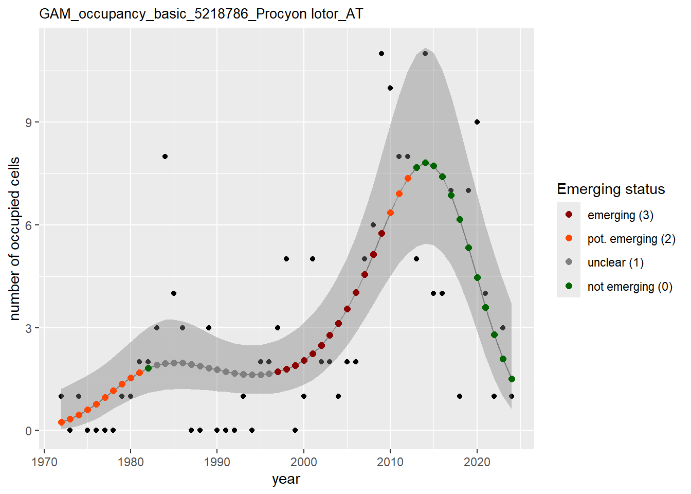
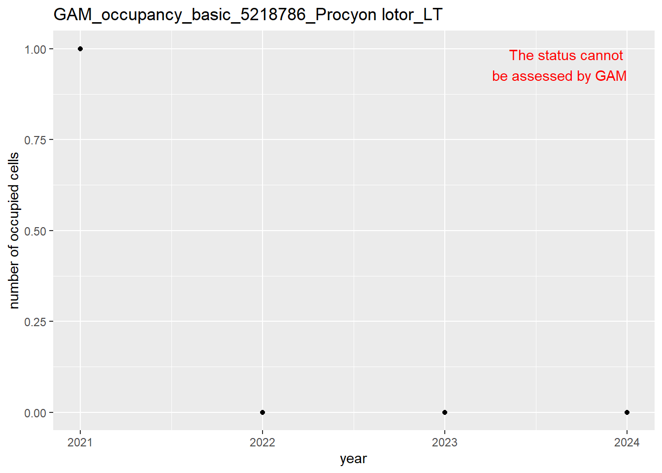
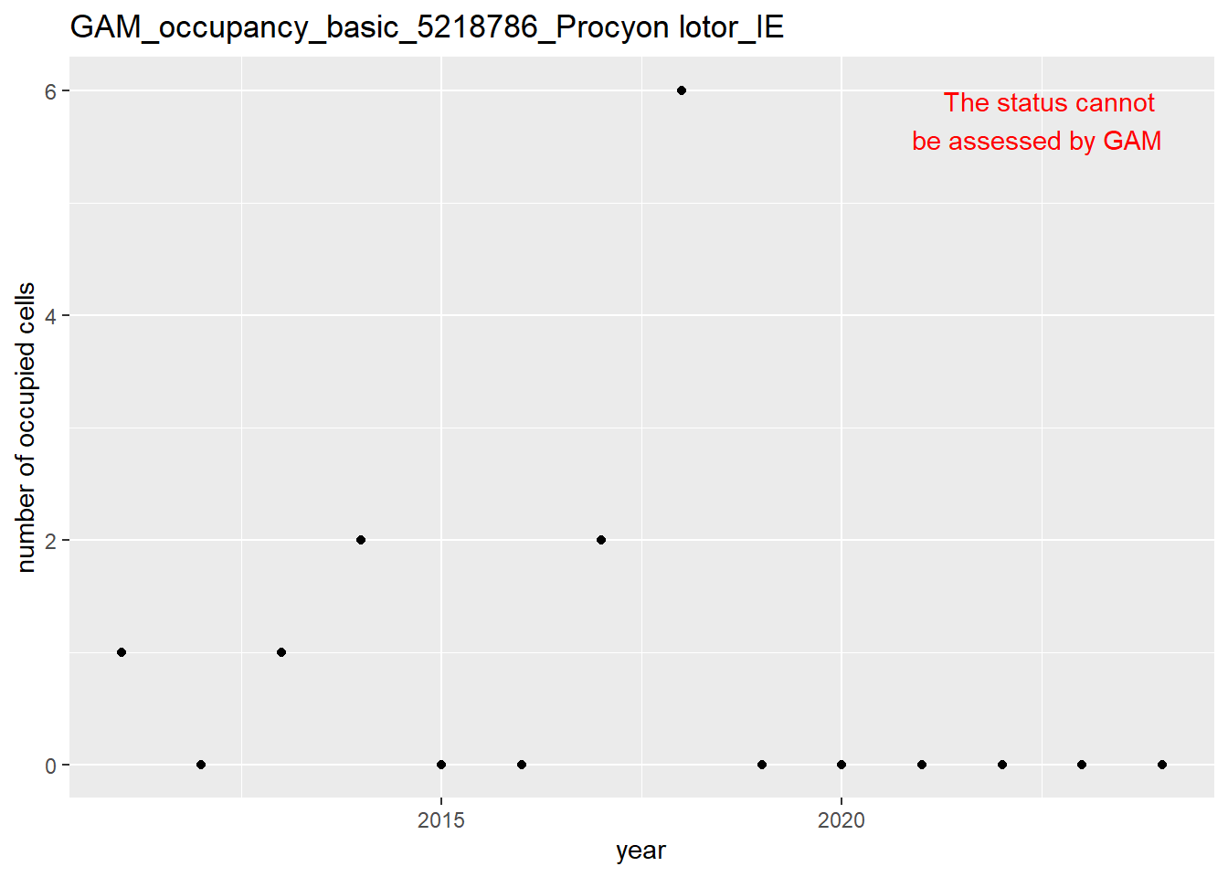
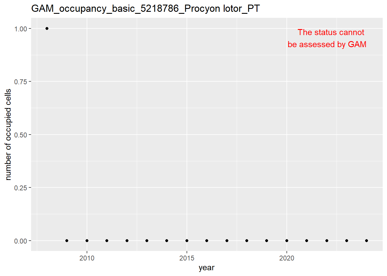
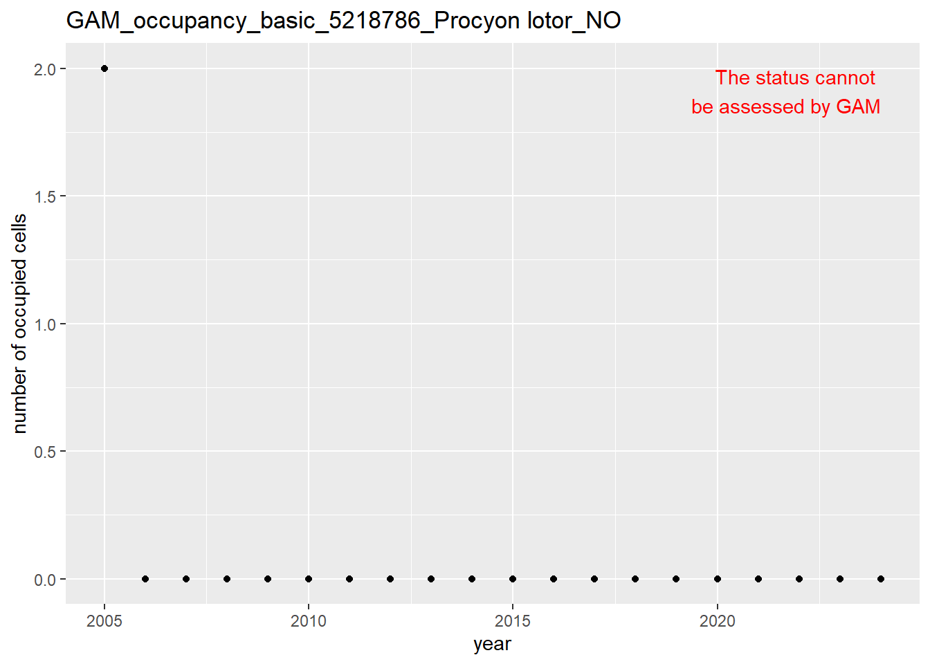
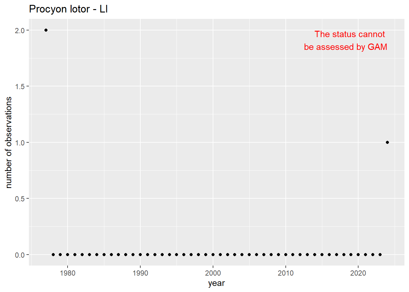
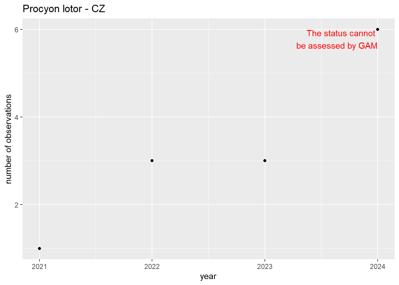
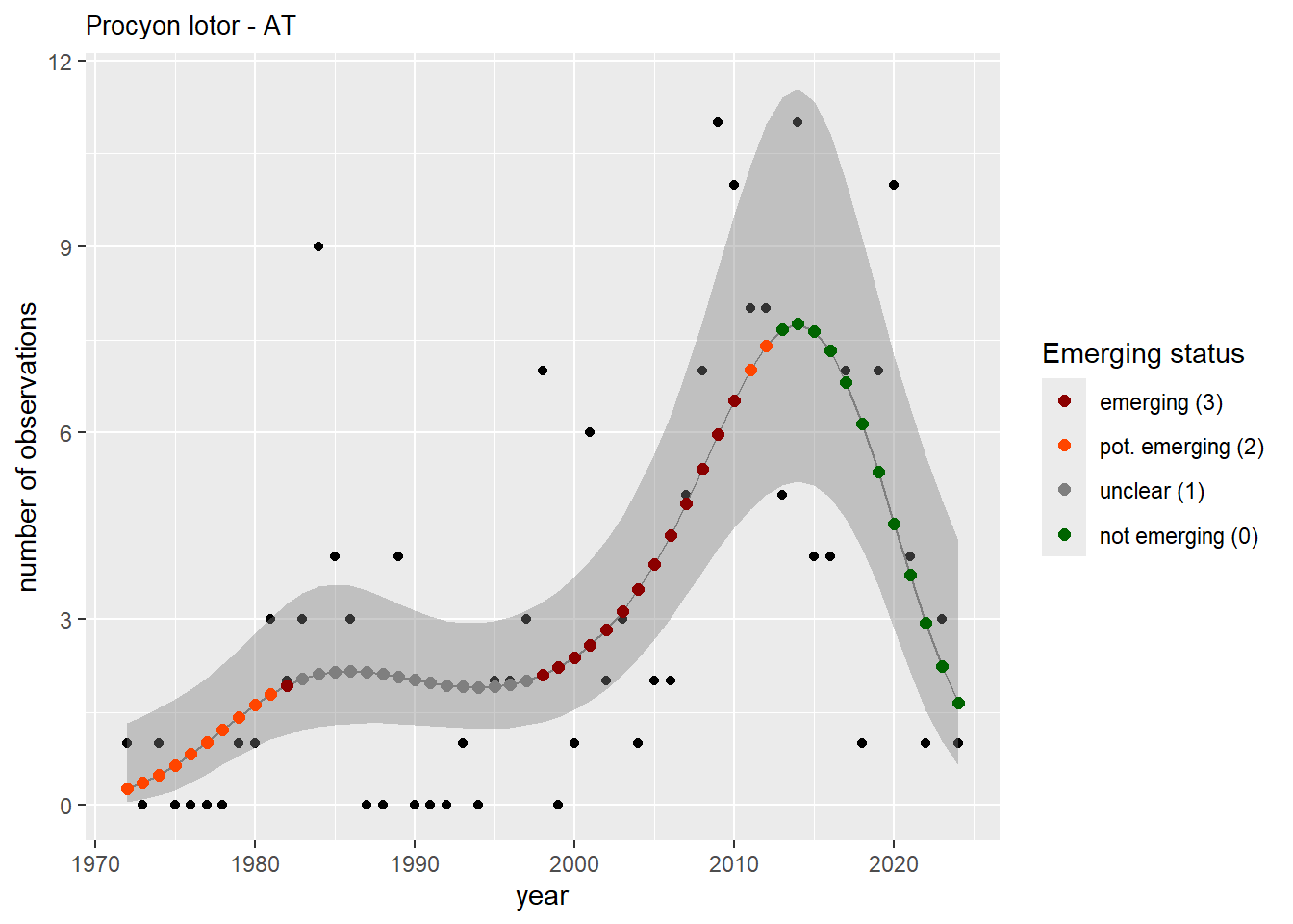
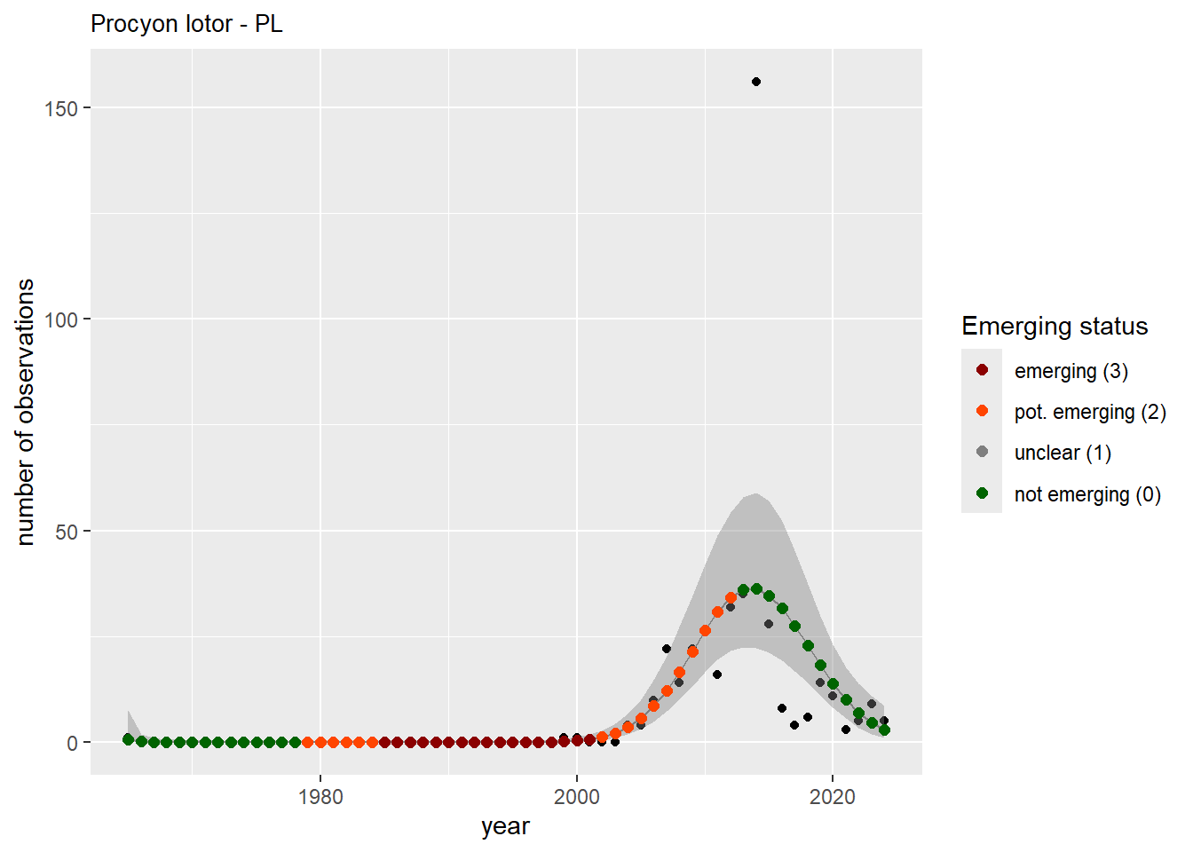
names(gam_ncells) <- countrycodePlease go to ./data/output/GAM_outputs to download the plots shown in this section.
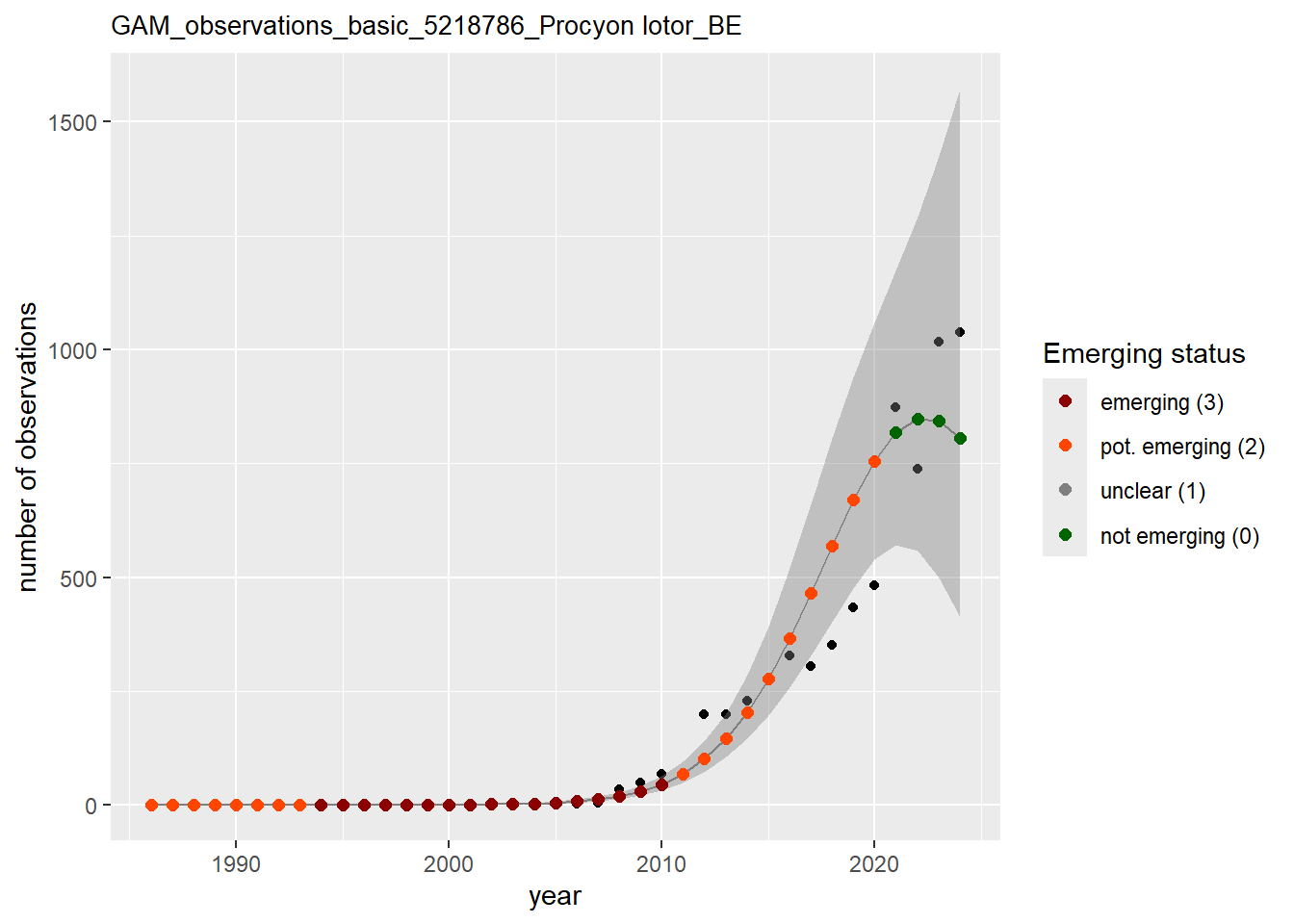
In this section we show the plots as returned by apply_gam(). Plot titles could be quite long. Folder: ./data/output/GAM_outputs/long_titles.
purrr::walk(gam_occs, function(country) {
  purrr::walk(country, function(x) print(x$plot))
  }
)


purrr::walk(gam_ncells, function(country) {
  purrr::walk(country, function(x) print(x$plot))
  }
)


We show and save plots with the species only as title. We save them in sub folder ./data/output/GAM_outputs/short_title.
purrr::iwalk(gam_occs, function(x, country) {
  purrr::iwalk(x, function(y, sp) {
    y$plot <- y$plot + ggplot2::ggtitle(label = paste(sp, "-", country))
    ggplot2::ggsave(
      filename = here::here(
        "data",
        "output",
        "GAM_outputs",
        "short_title",
        paste0("occurrences_", sp, "_", country, ".png")),
      plot = y$plot,
      width = plot_dimensions$width,
      height = plot_dimensions$height,
      units = "px"
    )
    print(y$plot)
  })
})


We do the same for the measured occupancy (number of occupied grid cells).
purrr::iwalk(gam_ncells, function(x, country) {
  purrr::iwalk(x, function(y, sp) {
    y$plot <- y$plot + ggplot2::ggtitle(label = paste(sp, "-", country))
    ggplot2::ggsave(
      filename = here::here(
        "data",
        "output",
        "GAM_outputs",
        "short_title",
        paste0("occupancy_", sp, "_", country, ".png")),
      plot = y$plot,
      width = plot_dimensions$width,
      height = plot_dimensions$height,
      units = "px"
    )
    print(y$plot)
  })
})


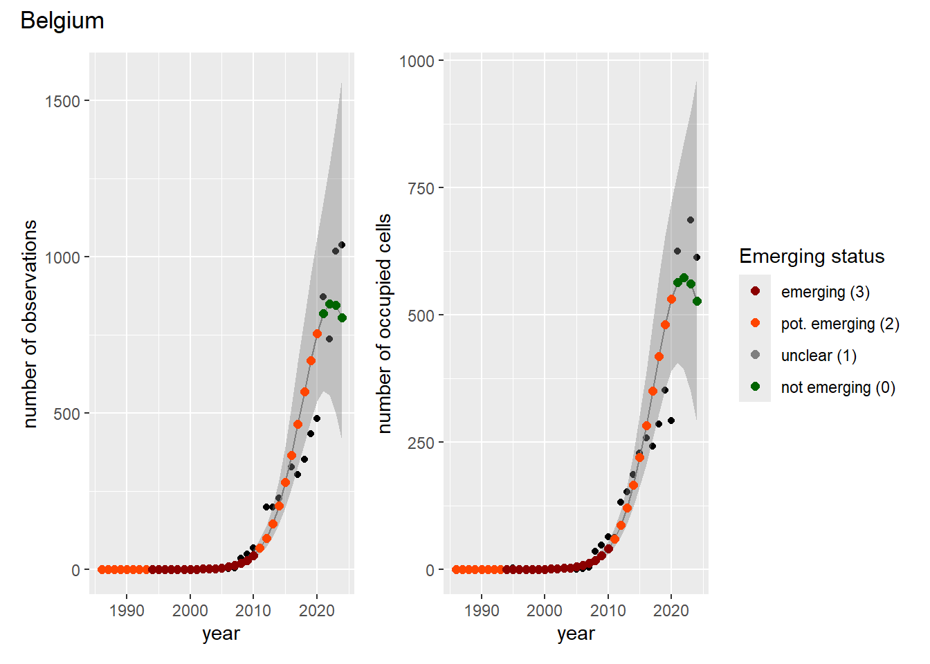
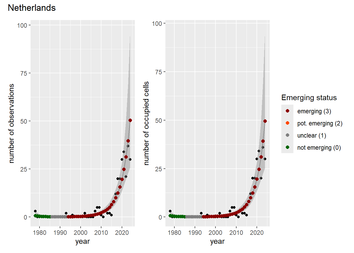
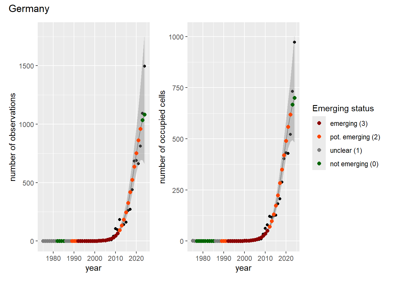
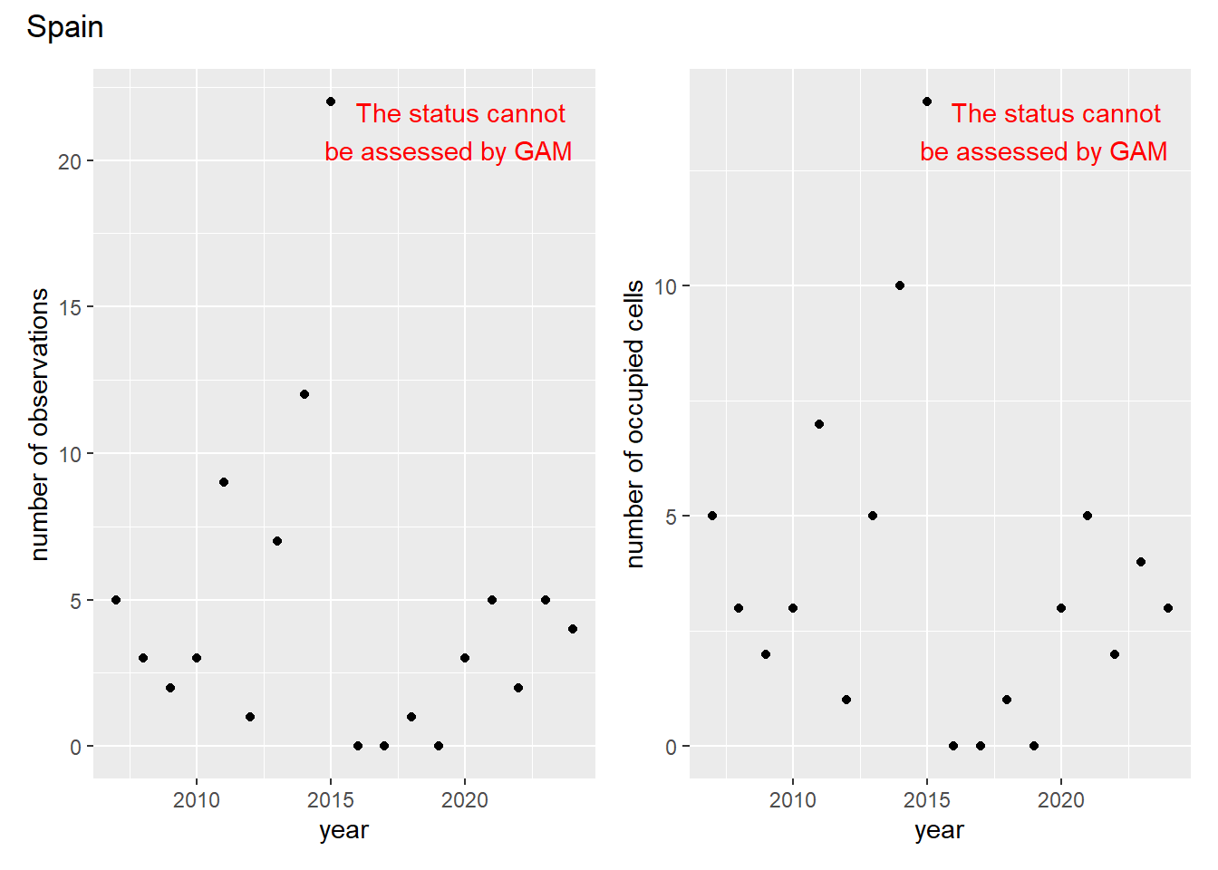
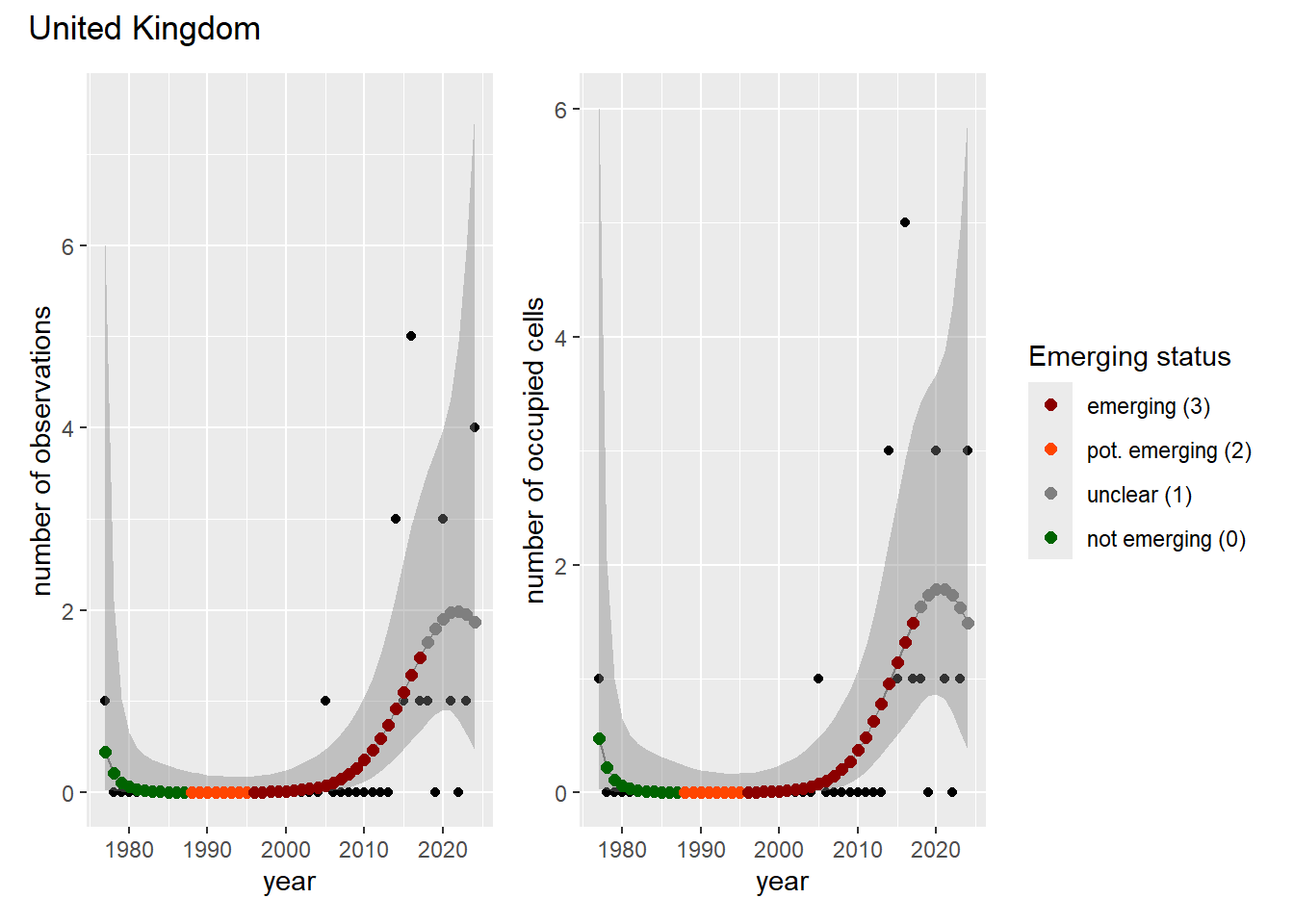
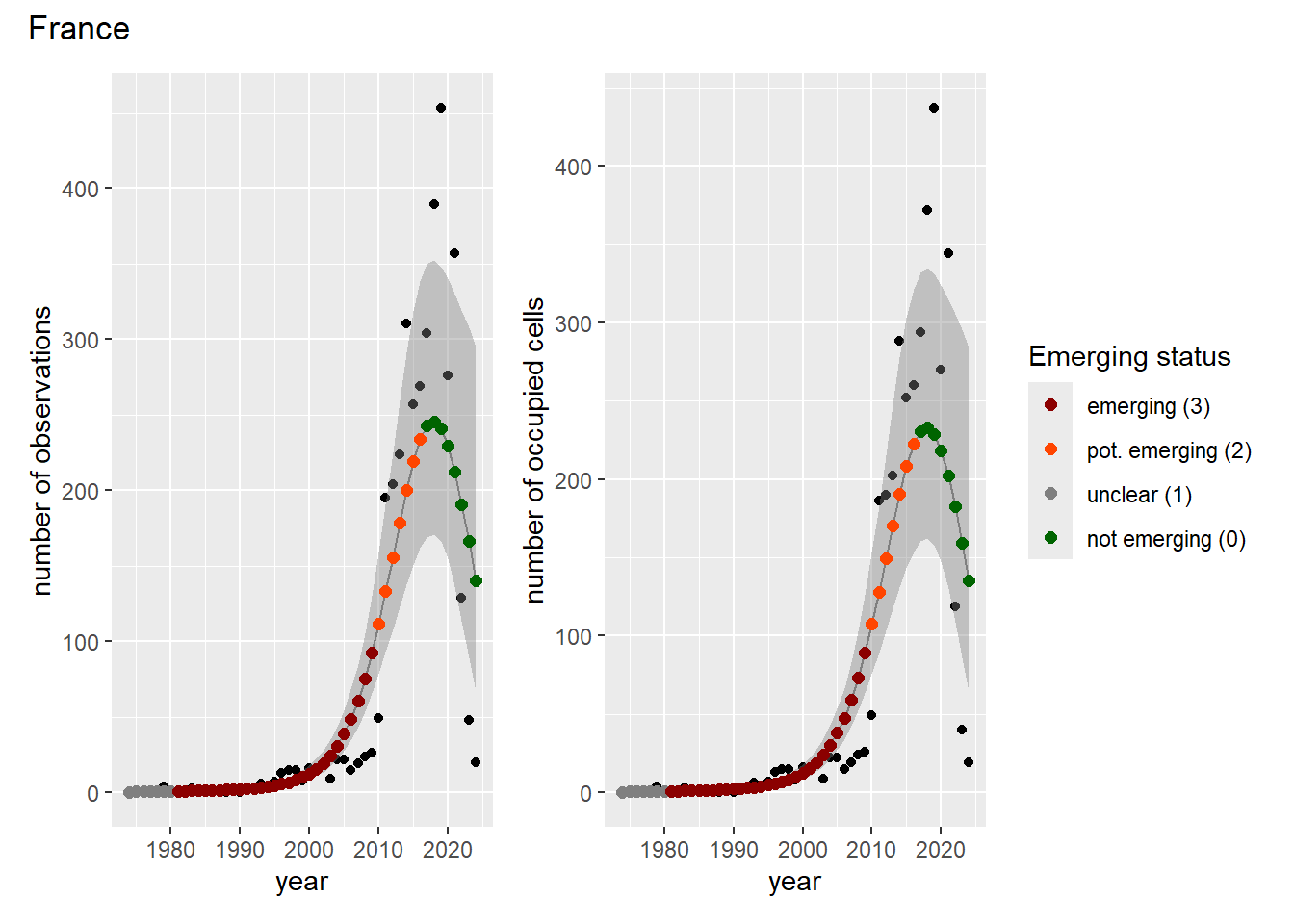
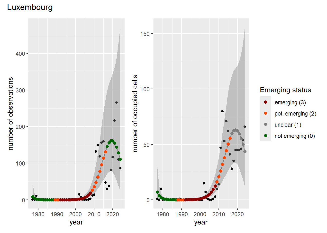
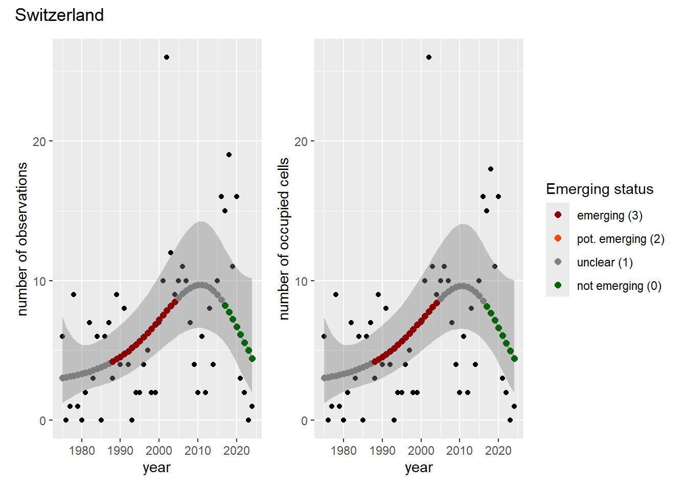
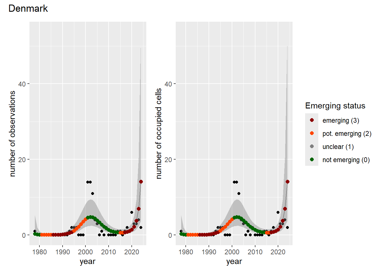
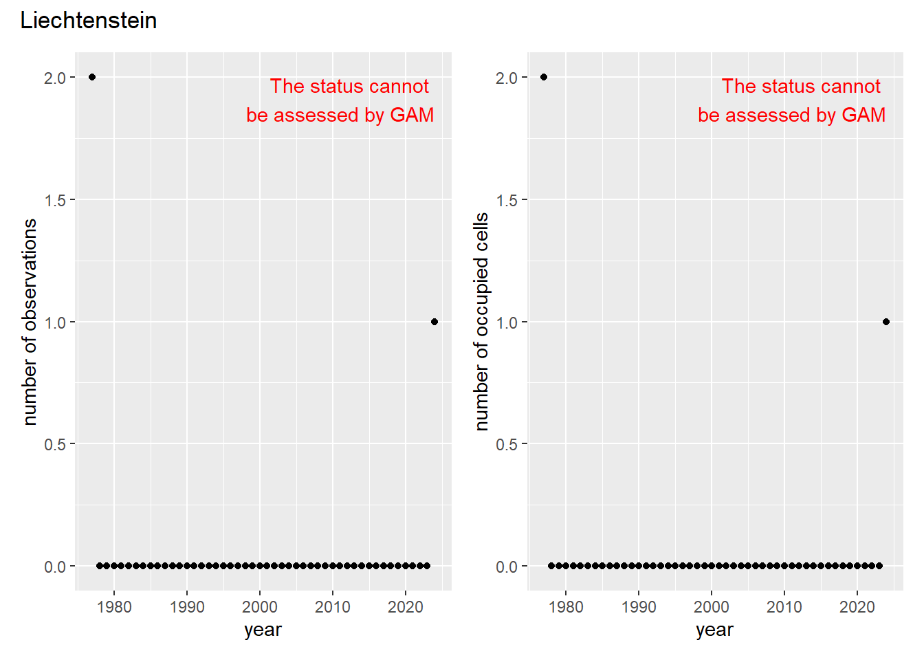
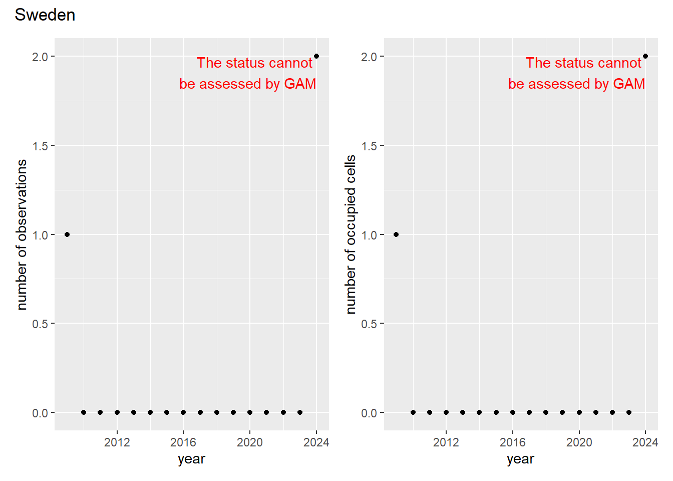
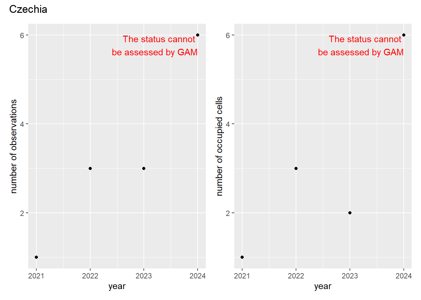
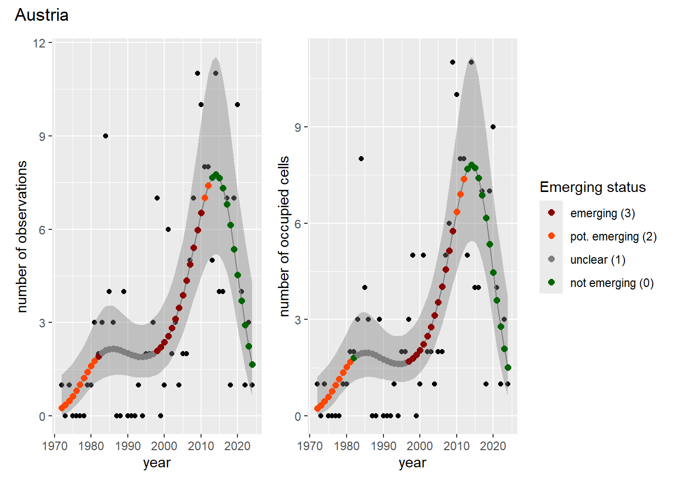
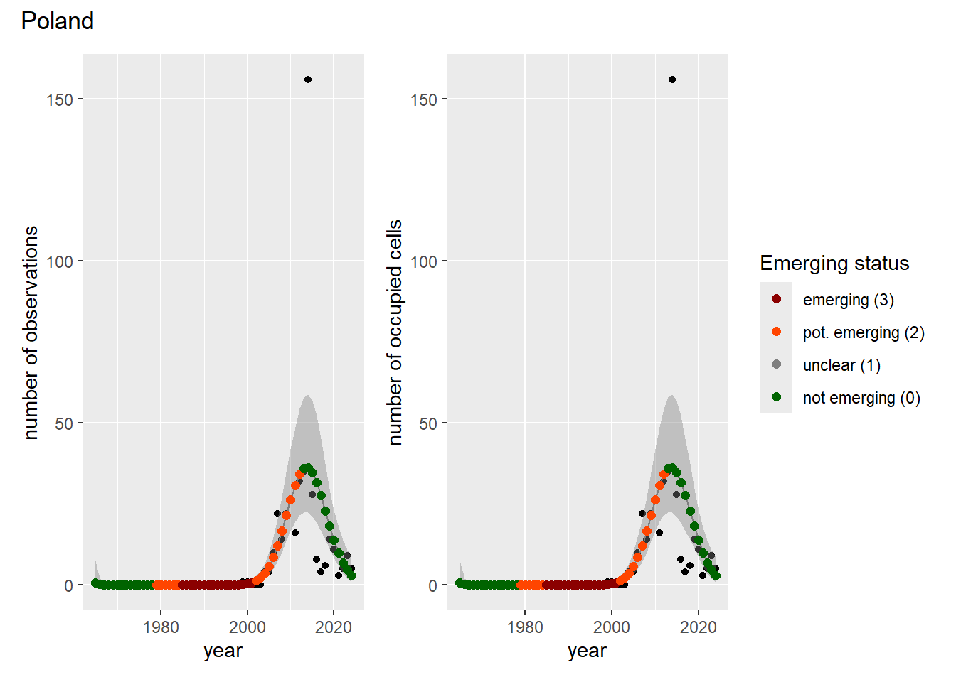
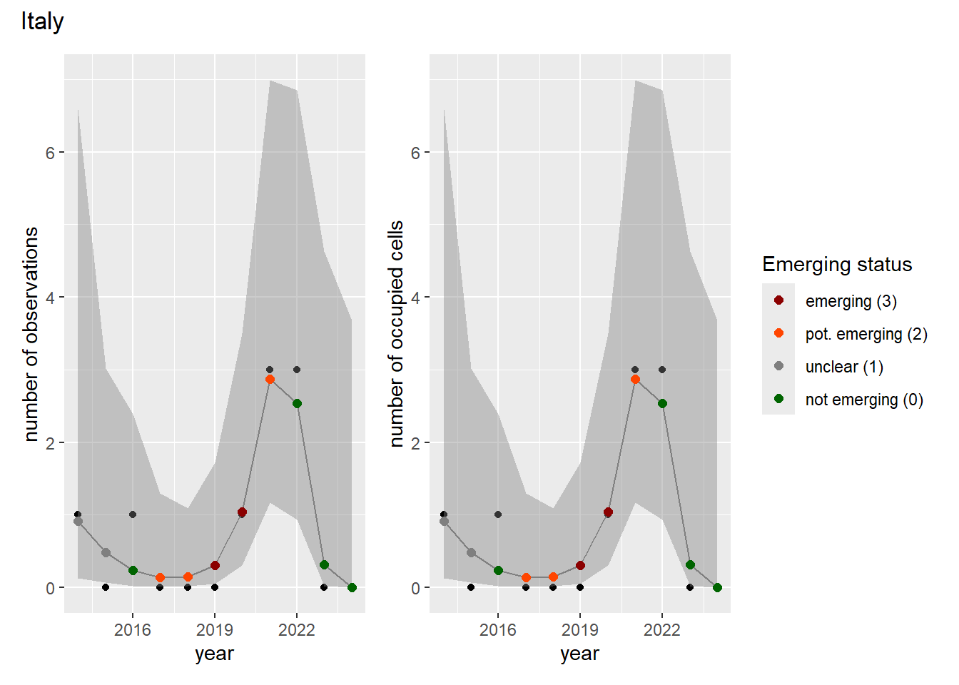
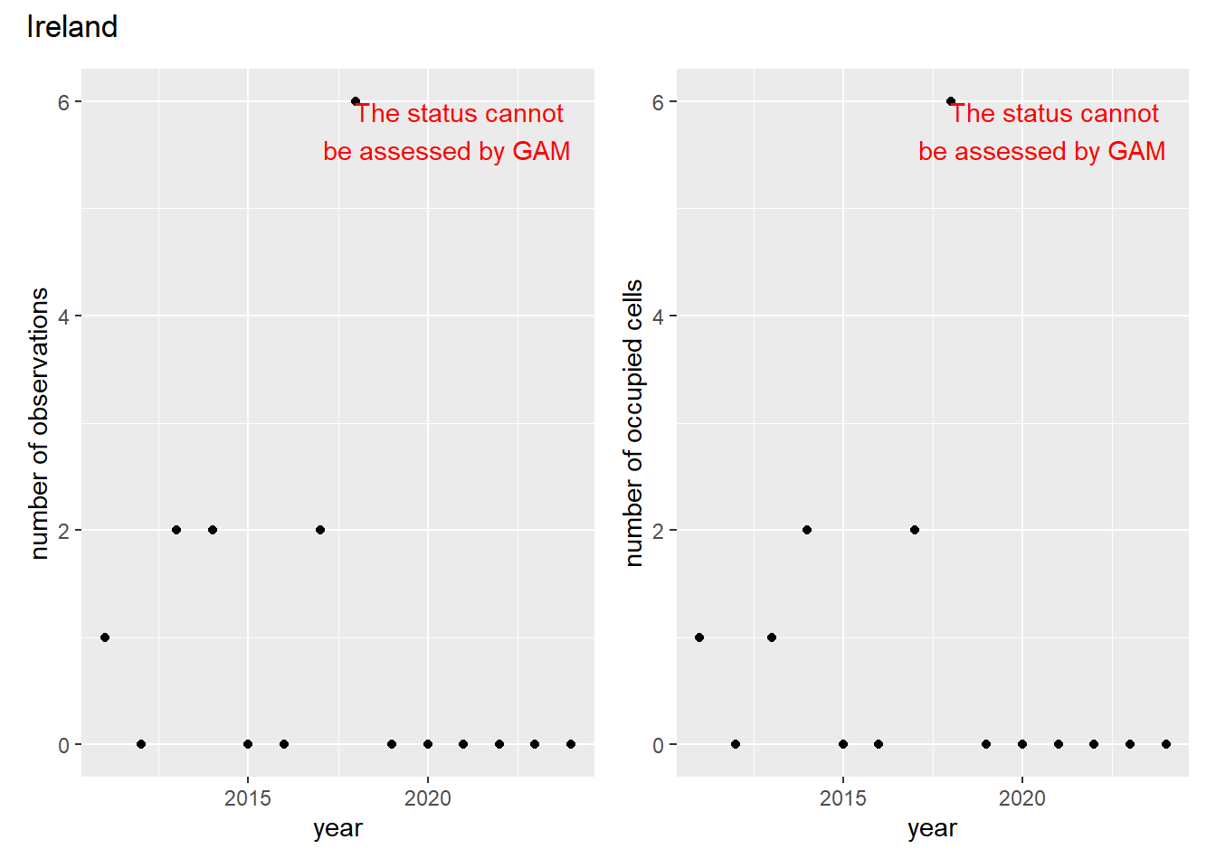
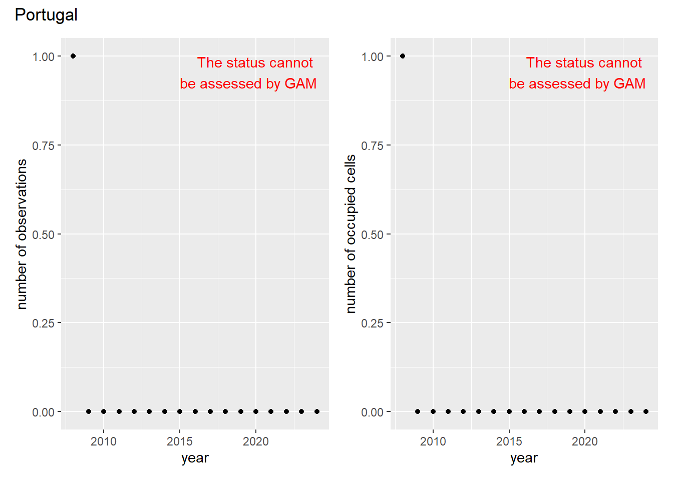
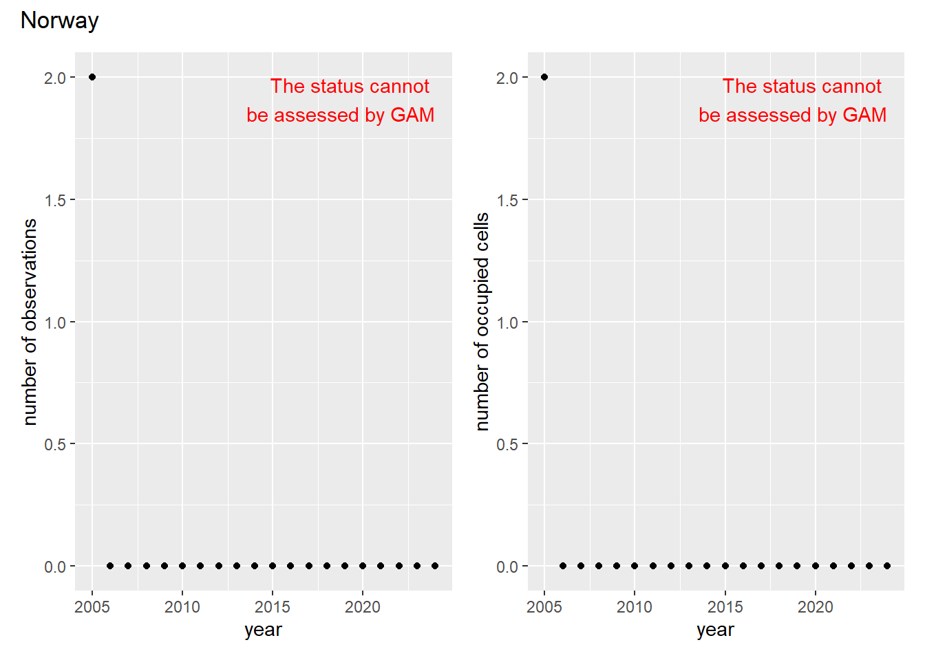
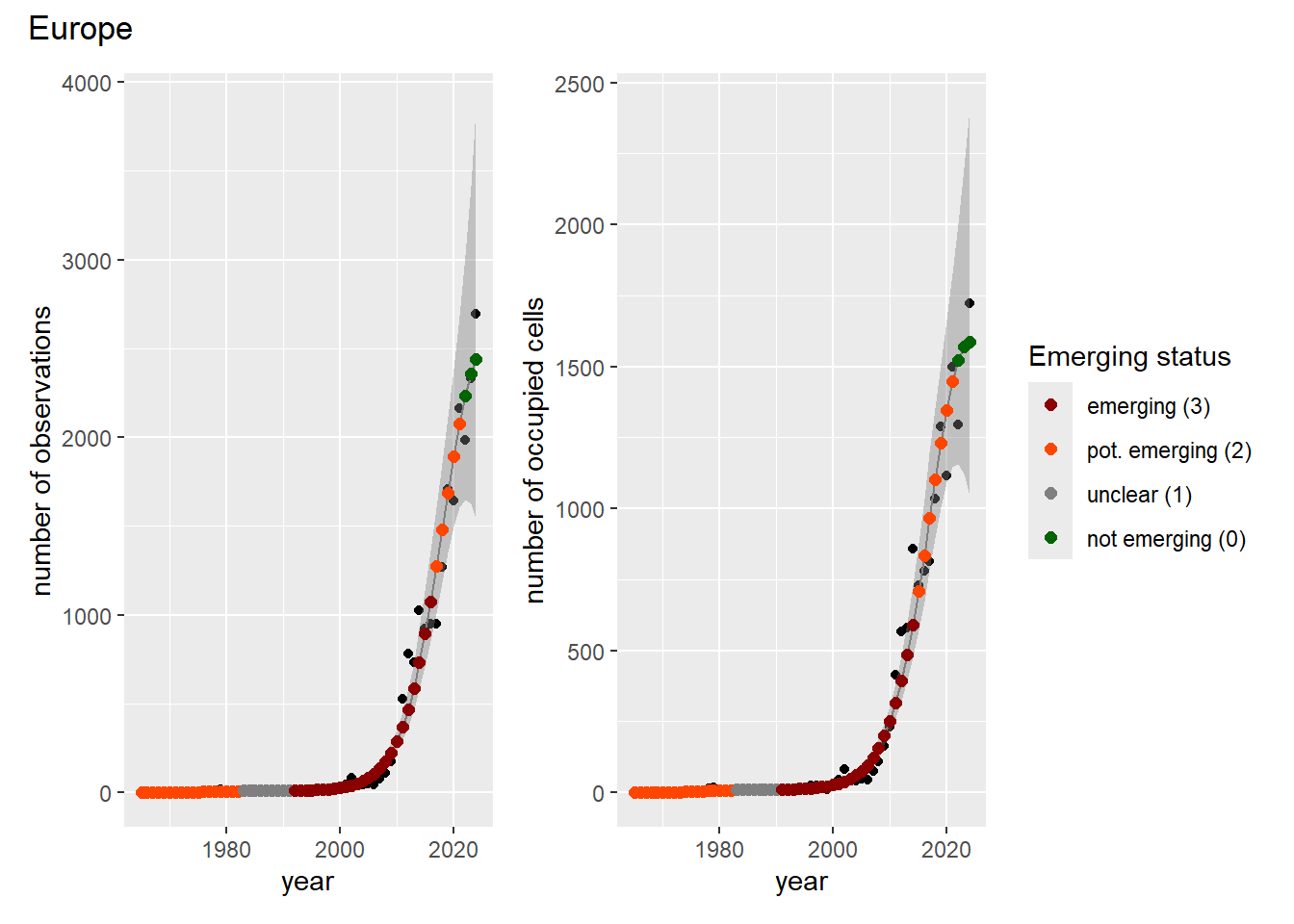
For each country, we can show the plots of the number of occurrences and the measured occupancy next to each other. We use the full country name. Plots are saved in subfolder ./data/output/GAM_outputs/plots_for_countries.
# Transform gam_occs and gam_ncells into a list of lists
gam_countries <- purrr::map(
  countrycode,
  function(code) {
    purrr::map2(
      gam_occs[[code]],
      gam_ncells[[code]],
      function(x, y) list(occurrences = x, ncells = y)
    )
  }
)
names(gam_countries) <- countrycode
# Create a grid of plots for each country
purrr::walk2(
  gam_countries,
  countrycode,
  function(country, code) {
    purrr::walk(country, function(x) {
      # Remove title
      x$occurrences$plot <- x$occurrences$plot + ggplot2::ggtitle(NULL)
      x$ncells$plot <- x$ncells$plot + ggplot2::ggtitle(NULL)
      p <- patchwork::wrap_plots(x$occurrences$plot,
                                 x$ncells$plot,
                                 nrow = 1,
                                 ncol = 2) +
        # Unify legends
        patchwork::plot_layout(guides = 'collect') +
        # Add general title
        patchwork::plot_annotation(
          title = countries$country_name[countries$countrycode == code]
        )
      ggplot2::ggsave(
        filename = here::here(
          "data",
          "output",
          "GAM_outputs",
          "plots_for_countries",
          paste0(code, "_grid.png")),
        plot = p,
        width = plot_dimensions$width,
        height = plot_dimensions$height,
        units = "px"
      )
      print(p)
    })
  }
)